energies Article
A Hierarchical Method for Transient Stability Prediction of Power Systems Using the Confidence of a SVM-Based Ensemble Classifier Yanzhen Zhou 1, *, Junyong Wu 1 , Zhihong Yu 2 , Luyu Ji 1 and Liangliang Hao 1 1 2
*
School of Electrical Engineering, Beijing Jiaotong Univerisity, Beijing 100044, China;
[email protected] (J.W.);
[email protected] (L.J.);
[email protected] (L.H.) China Electric Power Research Institute, Beijing 100192, China;
[email protected] Correspondence:
[email protected]; Tel.: +86-10-5168-5209
Academic Editor: Neville R. Watson Received: 12 June 2016; Accepted: 8 September 2016; Published: 27 September 2016
Abstract: Machine learning techniques have been widely used in transient stability prediction of power systems. When using the post-fault dynamic responses, it is difficult to draw a definite conclusion about how long the duration of response data used should be in order to balance the accuracy and speed. Besides, previous studies have the problem of lacking consideration for the confidence level. To solve these problems, a hierarchical method for transient stability prediction based on the confidence of ensemble classifier using multiple support vector machines (SVMs) is proposed. Firstly, multiple datasets are generated by bootstrap sampling, then features are randomly picked up to compress the datasets. Secondly, the confidence indices are defined and multiple SVMs are built based on these generated datasets. By synthesizing the probabilistic outputs of multiple SVMs, the prediction results and confidence of the ensemble classifier will be obtained. Finally, different ensemble classifiers with different response times are built to construct different layers of the proposed hierarchical scheme. The simulation results show that the proposed hierarchical method can balance the accuracy and rapidity of the transient stability prediction. Moreover, the hierarchical method can reduce the misjudgments of unstable instances and cooperate with the time domain simulation to insure the security and stability of power systems. Keywords: transient stability prediction; support vector machine (SVM); ensemble classifier; machine learning; confidence level; hierarchical method; power systems
1. Introduction With the continuous growth of electricity demand and the enlargement of the power system interconnection scale, power systems are becoming increasingly complex and have been forced to operate closer to their stability limits. Hence, ensuring the security of power systems has become more challenging. Transient instability has historically been the dominant stability problem in power systems [1]. Therefore, the study on the transient stability has great significance for the secure and stable operation of power systems. Transient, or large-disturbance rotor angle stability, refers to the ability of an interconnected power system to maintain synchronism after a severe disturbance [1], and the relevant literature is rich. Time domain simulation is the most traditional transient stability analysis method. However this method depends on exact models and parameters, and it is time-consuming which makes it hard to apply online. Other traditional methods, such as the transient energy function method and extended equal-area criterion, have model limitations which makes it hard for them to give efficient and precise results for large-scale power systems. Recently, the machine learning techniques, with high computing speed and precision, as well as the capacity of mining the potential useful information Energies 2016, 9, 778; doi:10.3390/en9100778
www.mdpi.com/journal/energies
Energies 2016, 9, 778
2 of 20
from among massive sets of data, have been used to predict the transient stability [2–19]. The transient stability prediction can be treated as a two-class classification (stable and unstable) problem and solved by machine learning methods. A set of appropriate features/attributes is selected to generate the offline training sets, then an appropriate classification method is utilized to predict the transient stability status. There are two kinds of machine learning-based methods with different types of inputs [2]. One uses pre-fault steady-state variables as the original data, the machine learning method will be used to build the mapping between the steady-stable variables and the transient stability status with respect to an anticipated but not yet occurred contingency [2–5]. Once the current status is identified as insecure, preventive control can be carried out to modify the system to a secure state. However, when a serious fault happens, or failure of primary relay protection, the power system may still be unstable even if the preventive control has been conducted. Therefore we should emphasize importance of the study on transient stability prediction using post-fault responses. Because the post-fault responses carry information about the influence of the faults on the power system, the prediction is independent of the faults. This arises the second way of transient stability prediction based on machine learning techniques. With the development of wide-area measurement systems, the dynamic response of power systems after a disturbance can be measured by phasor measurement units, which provides data support for post-fault transient stability prediction. However, it brings forward strict requirements regarding the prediction accuracy and speed because a fault has already occurred. Recently, the construction of input data and the improvement of machine learning methods to increase the accuracy have been the main research focus. Methods such as neural networks [6–8], decision trees (DTs) [9–11], support vector machines (SVMs) [12–15], fuzzy theory [16,17] and some ensemble classifiers [18,19] had been used for post-fault transient stability analysis. In fact, a classifier should possess high prediction accuracy, but it is also important to estimate the credibility of each classification result, or the confidence level. The existing transient stability prediction only provides a prediction result but seldom considers the confidence level. When two stable results are provided by a classifier, one with lower confidence whereas the other with higher confidence, these two situations should be treated differently. In [14], the results are divided into credible and incredible simply based on the SVM results, but lack further research on the definition and application of confidence indices. The post-fault dynamic responses vary with time, and the selection of the duration time of the response data, called response time in this paper, is always a problem that needs to be solved for post-fault transient stability prediction. The sooner the prediction is completed, the longer the time available to take actions to avoid a possible collapse is [13]. Thus, selecting too long a response time cannot meet the requirements of online application. However, the responses with little duration time may still not display distinguishing characteristics, which increases the difficulty to achieve high accurate prediction, so the accuracy and speed are contradictory. In the literature, a relative optimal response time will be determined by the comparison between the accuracy and time of different classifiers with different response times. The selections of response times are different, e.g., 50 ms in [12], 150 ms and 300 ms in [17], 200 ms in [11]. Therefore it is hard to draw definite conclusions about that how long the best response time for any power system is. Among the various machine learning methods, SVM has demonstrated better performance in transient stability prediction. The SVM classifier can not only provide the prediction results, but also give out the “distance” between the instance and stable boundary [14], which can be further used to define the confidence index. Based on the aforementioned analysis, we propose in this paper a SVM-based ensemble classifier and its confidence evaluation index. Most importantly, the proposed confidence index provides the credibility evaluation of transient stability prediction results and a new solution for the selection of response time, helping to construct a comprehensive hierarchical method which can balance the accuracy and rapidity.
Energies 2016, 9, 778
3 of 20
The rest of this paper is organized as follows: Section 2 introduces the generation of datasets Energies 2016, 9, 778 3 of 20 for transient stability prediction. Section 3 introduces the SVM-based ensemble classifier and its confidence index. Based on the contents in Sections 2 and 3, the proposed hierarchical method will be confidence index. Based on the contents in Sections 2 and 3, the proposed hierarchical method will introduced in Section 4. Results and Discussions of comprehensive case studies on 16-machine 68-bus be introduced in Section 4. Results and Discussions of comprehensive case studies on 16‐machine 68‐ power system are conducted in Section 5. The conclusions are given in Section 6. bus power system are conducted in Section 5. The conclusions are given in Section 6. 2. Generation of Dataset 2. Generation of Dataset In terms of machine learning-based method for transient stability prediction, the first step is to In terms of machine learning‐based method for transient stability prediction, the first step is to generate the original dataset, shown in Figure 1. generate the original dataset, shown in Figure 1.
Figure 1. Dataset for machine learning‐based transient stability prediction.
Figure 1. Dataset for machine learning-based transient stability prediction.
Generally, the transient stability dataset is generated by the time domain simulations [19]. When
Generally, the transient stability dataset is generated by the time domain simulations [19]. When a a power system is determined, the uncertainties associated with load levels, network configurations, fault types, locations and clearing times need to be modeled, then the time domain simulations will power system is determined, the uncertainties associated with load levels, network configurations, i ∈ {+1,−1} is will fault be carried out to determine whether the system is transient stable or not. In Figure 1, y types, locations and clearing times need to be modeled, then the time domain simulations the transient stability label, y i = +1 and yi = −1 represent the stable and unstable respectively. Finally, be carried out to determine whether the system is transient stable or not. In Figure 1, yi ∈ {+1,−1} is n instances in total with their transient stability labels are obtained. the transient stability label, yi = +1 and yi = −1 represent the stable and unstable respectively. Finally, Massive amounts of data will be generated during the time domain simulation, e.g., the generator n instances in total with their transient stability labels are obtained. electromagnetic powers, rotor angles and speeds, bus voltages and transmission line powers. Using Massive amounts of data will be generated during the time domain simulation, e.g., the generator all the variables will make the scale of the dataset too large, and even cause a “dimension disaster” electromagnetic powers, rotor angles and speeds, bus voltages and transmission line powers. Using problem. Thus it is necessary to extract some important features to describe the instances. all the variables will make the scale of the dataset too large, and even cause a “dimension Transient stability, or large‐disturbance rotor angle stability, refers to the ability of all disaster” the problem. Thus itto ismaintain necessary to extract after somea important features to describethe thegenerator instances. generators synchronism severe disturbance. Therefore dynamic responses carry important information for transient stability prediction. Varieties of input features Transient stability, or large-disturbance rotor angle stability, refers to the ability of all the generators have been utilized in previous research. From the perspective of whether the number of features is to maintain synchronism after a severe disturbance. Therefore the generator dynamic responses carry related to the scale of the power system, the input features can be divided into the component features important information for transient stability prediction. Varieties of input features have been utilized and system features. The component features are the variables of individual components, e.g., the in previous research. From the perspective of whether the number of features is related to the scale rotor angles, electromagnetic powers of generators, etc. The system features are the combined of the power system, the input features can be divided into the component features and system variables that are computed by the variables of multiple components. The most major characteristic features. The component features are the variables of individual components, e.g., the rotor angles, of the system features is that the feature number is independent of the power system scale. electromagnetic powers of generators, etc. The system features are the combined variables that are On the basis of the related literature and our comprehension of transient stability, we utilized computed by the variables of multiple components. The most major characteristic of the system the statistics of the generator variables to construct the input features, shown in Table 1. The statistical features can be viewed as the system features and their amount is independent of the power system features is that the feature number is independent of the power system scale. scale. All the input features are defined in the following subsections. On the basis of the related literature and our comprehension of transient stability, we utilized the statistics of the generator variables to construct the input features, shown in Table 1. The statistical features can be viewed as the system features and their amount is independent of the power system scale. All the input features are defined in the following subsections.
Energies 2016, 9, 778 Energies 2016, 9, 778
4 of 20
Table 1. Construction of the input features. COI: centre of inertia.
4 of 20
Feature Description Feature Description Table 1. Construction of the input features. f1 Average{Pmi(tb)} f18 Max{ῶi(tk)} + Min{ῶi(tk)} f 2 Average{P ei (t FOT )/P mi (t FOT )} f 19 Coefficient of variation{ῶ Feature Description Feature Description i(tk)} f3 Max{Pei(tFOT)/Pmi(tFOT)} f20 αCOI(tk) f1 Average{Pmi (tb )} f 18 Max{ω e i (tk )} + Min{ω e i (tk )} f 4 Min{P ei (t FOT )/P mi (t FOT )} f 21 Average{|ᾶ i(tk)|} f2 Average{Pei (tFOT )/Pmi (tFOT )} f 19 Coefficient of variation{ ω e i (tk )} Average{P (tk)/P miFOT (tk)} f22 f 20 Variance{ᾶ i(t(t k)} f 3 f5 Max{P )} αCOI ei (tFOTei)/P mi (t k) f 4 f6 Min{P (tkFOT αi (t ei (tFOT Max{P ei(tk)/P )/Pmi mi(t )} )} f23 f 21 Max{ᾶi(tAverage{|e k)} − Min{ᾶ i(tkk)|} )} f5 Average{Pei (tk )/Pmi (tk )} f 22 Variance{e αi (tk )} f7 Min{Pei(tk)/Pmi(tk)} f24 Max{ᾶi(tk)} + Min{ᾶi(tk)} f6 Max{Pei (tk )/Pmi (tk )} f 23 Max{e αi (tk )} − Min{e αi (tk )} (tk) (t )} f25 f Coefficient of variation{ᾶ k)} f 7 f8 Min{PδeiCOI (tk )/P Max{e αi (tk )} + Min{e αi(t 24 mi k i (tk )} Average{|δ̃ f26 f 25 Average{EK i(tk)} f 8 f9 δCOI (tk )i(tk)|} Coefficient of variation{e αi (tk )} e f 9 f10 Average{EK Average{| δi (t Variance{δ̃ i(t )} f27 f 26 Variance(EK i(tk)) i (tk )} kk)|} e f 10 f11 f Variance(EK Variance{ δ (t )} 27 i (ti(t k )) i k i(tk)} Max{δ̃i(tk)} − Min{δ̃ f28 Max{EKi(tk)} − Min{EK k)} e e f 11 f12 f Max{EK (t )} − Min{EK Max{ δ (t )} − Min{ δ (t )} 28 i k Max{δ̃ii(tkk)} + Min{δ̃ii(tkk)} f29 Max{EKi(tk)} + Min{EKi(tk)} i (tk )} f 12 f Max{EKi (tk )} + Min{EKi (tk )} Max{e δi (tk )} + Min{e δi (tk )} f13 Coefficient of variation{δ̃ i(tk)} f30 29 Coefficient of variation{EK i(tk)} f 13 f 30 Coefficient of variation{EKi (tk )} Coefficient of variation{e δi (tk )} ωCOI(t(tk) ) f31 f Max{dEK i/dt} − Min{dEKi/dt}|t = tk Max{dEK f 14 f14 ω COI k 31 i /dt} − Min{dEKi /dt}|t = tk Average{|ῶ (tkk)|} )|} f32 f 32 v(tk) v(tk ) f 15 f15 Average{|ω e ii(t f 16 f16 Variance{ ω e (t )} f δ (tk )GB−(tkδ) GB (tk ) Variance{ῶii(tkk)} f33 33 δGL(tkGL ) − δ f 17 f17 Max{ ω e (t )} − Min{ ω e (t )} f ω (tk )GB −(tω (t ) 34 GL i k i k Max{ῶi(tk)} − Min{ῶi(tk)} f34 ωGL(tk) − ω k) GB k 2.1. Generator Electromagnetic Powers 2.1. Generator Electromagnetic Powers Generator electromagnetic powers have been utilized to construct the input features [14]. Generator electromagnetic powers have been utilized to construct the input features [14]. The The power system is equilibrium in equilibrium before a fault occurs,and andthe theaverage averageof of all all the the generator power system is in before a fault occurs, generator electromagnetic powers reflects When a a fault electromagnetic powers reflects the the load load level level of of the the current current status. status. When fault occurs, occurs, the the electromagnetic power will suddenly change but the mechanical power cannot because of the inertia of electromagnetic power will suddenly change but the mechanical power cannot because of the inertia the governor. Thus the ratio of the electromagnetic and mechanical power of the i-th generator, Pei /Pmi , of the governor. Thus the ratio of the electromagnetic and mechanical power of the i‐th generator, reflects the relative variation of the i-th generator electromagnetic power following this fault. Figure 2 Pei/Pmi, reflects the relative variation of the i‐th generator electromagnetic power following this fault. shows the variation the Pei /P of aP16-machine 68-bus system (see system Section (see 5) forSection the unstable Figure 2 shows the of variation of ei/Pmi of a 16‐machine 68‐bus 5) for and the mithe stable cases. electromagnetic power is equal to the mechanical power of each generator a unstable and The stable cases. The electromagnetic power is equal to the mechanical power before of each fault occurs, that is Pei /Pmi = 1. When the fault occurs, the value of Pei /Pm will reduceeiand remain at a generator before a fault occurs, that is P ei/P mi = 1. When the fault occurs, the value of P /Pm will reduce low level until the fault is cleared. After the fault clearance, the value of Pei /Pmi reflects eithe /Pmirecovery reflects and remain at a low level until the fault is cleared. After the fault clearance, the value of P of the generator electromagnetic power. The value of Pei /Pmi will tend to 1 for the stable case. On the the recovery of the generator electromagnetic power. The value of P ei/P mi will tend to 1 for the stable contrary, when the system is stable, the value of Pei /Pmi of oneei/P generator is far away from 1. Therefore case. On the contrary, when the system is stable, the value of P mi of one generator is far away from 1. the value of Peivalue /Pmi can tobe identify theidentify transient stability status. Based on the statistics of Therefore the of Pbe ei/Pused mi can used to the transient stability status. Based on the generator electromagnetic powers, totally seven input features, f 1 –f 7 shown1in Table 1 are defined as statistics of generator electromagnetic powers, totally seven input features, f –f7 shown in Table 1 are the input features, where tb is the time before the fault occurs, tFOT is the occurrence time. defined as the input features, where t b is the time before the fault occurs, t FOTfault is the fault occurrence time.
Figure 2. The variation of P /Pmi of 16‐machine 68‐bus system: (a) unstable case; and (b) stable case. Figure 2. The variation of Peiei/P mi of 16-machine 68-bus system: (a) unstable case; and (b) stable case.
Energies 2016, 9, 778
5 of 20
Energies 2016, 9, 778
5 of 20
2.2. Generator Rotor Angles 2.2. Generator Rotor Angles Transient stability is dependent on the dynamics of generator rotor angles, which have been used as the input feature in many literatures [8,9,14,19]. The concept of reference is have widely used Transient stability is dependent on the dynamics of generator rotor centre angles, angle which been used as the input feature in many literatures [8,9,14,19]. The concept of reference centre angle is in transient stability assessments, and called the centre of inertia (COI) [20]. For an N-generator power widely used in transient stability assessments, and called the centre of inertia (COI) [20]. For an N‐ system, the COI reference of the rotor angle at t = tk after the fault clearance, δCOI (tk ), is: generator power system, the COI reference of the rotor angle at t = tk after the fault clearance, δCOI(tk), is: NN
NN
i =1i 1
1 ii = 1
δCOIδ(tCOI k) ∑MMi δi δi i((ttkk ))// ∑MMi i k )(t=
(1)(1)
where δi(tk) and Mi are the rotor angle and inertia coefficient of the i‐th generator at at t = tk after the where δi (tk ) and Mi are the rotor angle and inertia coefficient of the i-th generator at at t = tk after fault clearance. Besides, the COI reference of rotor speed and acceleration, ωCOI(tk) and αCOI(tk), are the fault clearance. Besides, the COI reference of rotor speed and acceleration, ωCOI (tk ) and αCOI (tk ), shown in Equations (2) and (3) respectively: are shown in Equations (2) and (3) respectively: dδ ω COI (tk ) dδ COI t =tk dt |t = t (t ) = COI
ωCOI
k
dt
(2) (2)
k
dωCOI α (tk )dω COI t =tk αCOI (tCOI ) = dt |t = tk k
(3) (3) dt In In Equations (2) and (3), the derivative can be calculated using a difference approximation. From Equations (2) and (3), the derivative can be calculated using a difference approximation. here on, the relative rotor angle, speed and acceleration of the i‐th generator in the COI frame at t = t k From here on, the relative rotor angle, speed and acceleration of the i-th generator in the COI after the fault clearance are δ = δ i(tk) − δ COI (t k ), ῶ i (t k ) = ω i (t k ) − ω COI (t k ) and ᾶ i (t k ) = α i (t k ) − α COI (t k ) δi (tk ) = δi (tk ) − δCOI (tk ), ω frame at t = tk after the fault clearance are e e i (tk ) = ωi (tk ) − ωCOI (tk ) and respectively. α e i (tk ) = αi (tk ) − αCOI (tk ) respectively. The kinetic energy of the i‐th generator, EKi(tk), can also be used for transient stability prediction. The kinetic energy of the i-th generator, EKi (tk ), can also be used for transient stability prediction. It is defined as follows: It is defined as follows: 11 EKiEK (tk )(t=) M e i (tk ))22 i (ω (4)(4) i k i (ωi (t k )) 22M
Figures 3–6 show the variations of all the generator rotor angles, speeds, accelerations and kinetic Figures 3–6 show the variations of all the generator rotor angles, speeds, accelerations and energy of the 16-machine 68-bus system after the fault clearance. When the system is stable, the values kinetic energy of the 16‐machine 68‐bus system after the fault clearance. When the system is stable, of the rotor angles, speeds, accelerations and kinetic energy are low. However, the values of these the values of the rotor angles, speeds, accelerations and kinetic energy are low. However, the values quantities drastically. This inspires usinspires to extract theextract statistical features, such as maximum, quantities change drastically. This us to the statistical features, such as of these change minimum, variance etc. of the post-disturbance trajectories to construct the input features. Therefore, maximum, minimum, variance etc. of the post‐disturbance trajectories to construct the input features. based on the statistics of the aforementioned rotor angles, speeds, accelerations, kinetic energy, 24 input Therefore, based on the statistics of the aforementioned rotor angles, speeds, accelerations, kinetic features, f 8 –f 31 shown in Table are utilized for transient stability prediction. energy, 24 input features, f 8–f311, shown in Table 1, are utilized for transient stability prediction.
Figure 3. Generator rotor angles of 16‐machine 68‐bus system: (a) unstable case; and (b) stable case. Figure 3. Generator rotor angles of 16-machine 68-bus system: (a) unstable case; and (b) stable case.
Energies 2016, 9, 778 Energies 2016, 9, 778 Energies 2016, 9, 778 Energies 2016, 9, 778
6 of 20 6 of 20 6 of 20 6 of 20
Figure 4. Generator rotor speeds of 16‐machine 68‐bus system: (a) unstable case; and (b) stable case. Figure 4. Generator rotor speeds of 16-machine 68-bus system: (a) unstable case; and (b) stable case. Figure 4. Generator rotor speeds of 16‐machine 68‐bus system: (a) unstable case; and (b) stable case. Figure 4. Generator rotor speeds of 16‐machine 68‐bus system: (a) unstable case; and (b) stable case.
Figure 5. Generator rotor accelerations of 16‐machine 68‐bus system: (a) unstable case; and (b) stable case.
Figure 5. Generator rotor accelerations of 16‐machine 68‐bus system: (a) unstable case; and (b) stable case. Figure 5. Generator rotor accelerations of 16-machine 68-bus system: (a) unstable case; and (b) stable case. Figure 5. Generator rotor accelerations of 16‐machine 68‐bus system: (a) unstable case; and (b) stable case.
Figure 6. Generator kinetic energy of 16‐machine 68‐bus system: (a) unstable case; and (b) stable case.
Figure 6. Generator kinetic energy of 16‐machine 68‐bus system: (a) unstable case; and (b) stable case. Figure 6. Generator kinetic energy of 16‐machine 68‐bus system: (a) unstable case; and (b) stable case. Figure 6. Generator kinetic energy of 16-machine 68-bus system: (a) unstable case; and (b) stable case. 2.3. Other Useful Features
2.3. Other Useful Features 2.3. Other Useful Features Another useful quantity for transient stability prediction is the dot product of the rotor angles 2.3. Other Useful Features Another useful quantity for transient stability prediction is the dot product of the rotor angles and speed [17], v(t k): Another useful quantity for transient stability prediction is the dot product of the rotor angles and speed [17], v(t k): Another useful quantity for transient Nstability prediction is the dot product of the rotor angles and speed [17], v(tk): N (ω i (tk ) (δ i (tk ) δ i (0))) v(tk ) (5) and speed [17], v(tk ): i (tk ) (δ i (tk ) δ i (0))) iN 1 (ω v(tk N ) (5) (t ) δ (0))) i (tk ) (δ v(tk ) i 1 (ω (5)(5) i k i e e v ( t ) = ( ω e ( t ) × ( δ ( t ) − δ ( 0 +))) i i i ∑ k k k i 1 Where δ̃i(0+) and δ̃i(tk) are the relative rotor angle of the i‐th generator in the COI frame at the fault i =1 Where δ̃i(0+) and δ̃i(tkk) are the relative rotor angle of the i‐th generator in the COI frame at the fault clearing instant and t after the fault clearance, respectively, ῶi(tk) is the relative rotor speed of the i‐ Where δ̃ i(0+) and δ̃i(tk) are the relative rotor angle of the i‐th generator in the COI frame at the fault clearing instant and t k after the fault clearance, respectively, ῶi(tk) is the relative rotor speed of the i‐ e Where δi (0+) and e δi (tk after the fault clearance. are the relative rotor angle of the i-th generator in the COI frame at the fault th generator at t = t k )k after the fault clearance, respectively, ῶ clearing instant and t i(tk) is the relative rotor speed of the i‐ th generator at t = t k after the fault clearance. The generators with the fault biggest and smallest rotor acceleration be rotor the key generators clearing instant and t after the clearance, respectively, ω e ( tk ) is the may relative speed of the i-th k i th generator at t = t k after the fault clearance. The generators with the biggest and smallest rotor acceleration may be the key generators leading to the separation of rotor angles. In this research, these two generators are labelled as GL and generator at t = t after the fault clearance. k The generators with the biggest and smallest rotor acceleration may be the key generators leading to the separation of rotor angles. In this research, these two generators are labelled as GL and GB, respectively. Then rotor angle difference and speed difference of these two generators are also The generators with the biggest and smallest rotor acceleration may be the key generators leading leading to the separation of rotor angles. In this research, these two generators are labelled as GL and GB, respectively. Then rotor angle difference and speed difference of these two generators are also to used as the input features. the separation of rotor angles. In this research, these two generators are labelled as GL and GB, GB, respectively. Then rotor angle difference and speed difference of these two generators are also used as the input features. respectively. Then rotor angle difference and speed difference of these two generators are also used as used as the input features. the input features.
Energies 2016, 9, 778
7 of 20
Finally, the features shown in Table 1 form the 34 input features for transient stability prediction. These 34 features are the descriptions of all the generated instances shown in Figure 1. The dataset can be expressed as (xi , yi ), where i = 1, . . . , n, xi = [xij ]1×34 . To unify the original data from different Energies 2016, 9, 778 7 of 20 variables with different dimensions and accelerate the conversion speed, the original data are usually normalized using Equation (6): Finally, the features shown in Table 1 form the 34 input features for transient stability prediction. xij − min( xij ) These 34 features are the descriptions of all the generated instances shown in Figure 1. The dataset i ∗ x = (6) can be expressed as (xi, yi), where i = 1,…, n, xi = [xij]1×34. To unify the original data from different ij max( xij ) − min( xij ) variables with different dimensions and accelerate the conversion speed, the original data are usually i i normalized using Equation (6):
After the normalization, the original data are mapped into the range of [0, 1] and will be processed xij min( xij ) by the following machine learning methods the normalized data are also x * ij in Sectioni 3. For simplicity, (6) max( xij ) min( xij ) marked as xi = [xij ]1×34 in this paper. i i After the normalization, the original data are mapped into the range of [0, 1] and will be
3. Support Vector Machine-Based Ensemble Classifier and Its Confidence Evaluation processed by the following machine learning methods in Section 3. For simplicity, the normalized data are also marked as xi = [xij]1×34 in this paper.
3.1. Principle of Support Vector Machine 3. Support Vector Machine‐Based Ensemble Classifier and Its Confidence Evaluation
After the dataset (xi , yi ), or a set of instance-label pairs, is obtained, a machine learning method should be 3.1. Principle of Support Vector Machine selected and utilized to build the mapping between the input features and transient stability i, ywhich i), or a set of instance‐label pairs, is obtained, a machine learning method status y = f (x).After the dataset (x SVM algorithm, is based on the statistical learning and follows the principle of should be selected and utilized to build the mapping between the input features and transient stability the structural risk minimization [21], has been widely used for transient stability prediction [12–15]. status y = f(x). SVM algorithm, which is based on the statistical learning and follows the principle of In this research, SVM will be studied and used to build the transient stability classifier. the structural risk minimization [21], has been widely used for transient stability prediction [12–15]. Figure 7 shows the basic principle of SVM. The actual dataset is usually linearly inseparable In this research, SVM will be studied and used to build the transient stability classifier. Figure 7 shows the principle of into SVM. dataset is a usually linearly inseparable (Figure 7a), then this dataset isbasic transformed a The newactual space using nonlinear mapping, also called (Figure 7a), then this dataset is transformed into a new space using a nonlinear mapping, also called as the kernel function K(xi ,xj ). The transformed data may become linearly separable that much as the kernel function K(xi,xj). The transformed data may become linearly separable that much easier easier to find thethe best decision withthe the maximum classification the minimum to find best decision boundary boundary with maximum classification margin, margin, also the also minimum classification risk (Figure 7b). classification risk (Figure 7b).
Figure 7. Principle of support vector machine (SVM): (a) original data; and (b) transformed data.
Figure 7. Principle of support vector machine (SVM): (a) original data; and (b) transformed data. The best decision function y = f(x) can be expressed as:
The best decision function y = f (x) can be expressed as: N sv
f ( x ) sgn{ αi yisv K ( xisv , x ) b} N sv
(7)
i 1
∑
sv sv where sgn{} is sign function, N f (svx is the number of support vectors, x ) = sgn{ αi ysv } i K ( xi , x ) +i b is the i‐th support vectors and yisv is the corresponding label, b ∈ R, and αi = i is the Lagrange multiplier obtained from solving the 1 following optimization problem:
(7)
where sgn{} is sign function, Nsv is the number of support vectors, xi sv is the i-th support vectors and N 1N N sv sv sv sv minand α i αthe αi yi is the corresponding label, b ∈ R, α is multiplier obtained from solving the j yi yLagrange j K ( xi , x ) 2 i 1 ji1 i 1 following optimization problem: s.t. C α 0, i 1,..., l (8) sv
sv
sv
i
N sv
min
1 2
N sv
N sv
α y i
sv i
0
N sv
sv i 1 sv ∑ ∑ αi α j ysv i y j K ( x i , x ) − ∑ αi
i =1 j =1 where C ∈ R is the penalty parameter.
s.t.
i =1
C ≥ αi ≥ 0, i = 1, ..., l N sv
∑ αi ysv i =0
i =1
where C ∈ R is the penalty parameter.
(8)
Energies 2016, 9, 778
8 of 20
Common kernel functions include the polynomial, Gaussian radial basis function (RBF), and sigmoid function. In [22], it is verified that the RBF can approximate to any functions with arbitrary small error. In addition, many related articles had utilized the SVM with RBF for transient stability prediction [12–15]. Therefore the kernel function in this research is the RBF: K ( xsv i , x)
( ) x − xsv 2 i = exp − σ2
(9)
where σ ∈Energies 2016, 9, 778 R is the width of the Gaussian. 8 of 20 Two parameters, C and σ, need to be determined before the generation of the final SVM classifier. functions include be the found polynomial, Gaussian radial basis process function [12–15]. (RBF), and Generally, theCommon optimalkernel parameters should through a grid-search 3.2.
sigmoid function. In [22], it is verified that the RBF can approximate to any functions with arbitrary small error. In addition, many related articles had utilized the SVM with RBF for transient stability Confidence Evaluation of Support Vector Machine prediction [12–15]. Therefore the kernel function in this research is the RBF:
2 The nature of the aforementioned SVM decision of Equation (7) is a sign function. xfunction xisv sv K ( xis x ) exp or unstable from the output of SVM,(9) That means we can only know the instance but not the i , stable 2 σ distance between the instance and the optimal decision boundary. One method to improve the SVM output to awhere σ ∈ R is the width of the Gaussian. probabilistic output form is [23]:
Two parameters, C and σ, need to be determined before the generation of the final SVM classifier. Generally, the optimal parameters should be found through a grid‐search process [12–15]. P(C |x) = 1/(1 + e−g(x) ) +1
3.2. Confidence Evaluation of Support Vector Machine P(C−1 |x) = 1/(1 + eg (x) ) The nature of the aforementioned SVM decision function of Equation (7) is a sign function. That where P(Cmeans andcan P(C are the probabilities ofunstable an unknown identified +1 |x) we −1 |x) only know the instance is stable or from the instance output of xSVM, but not as the stable distance between the instance and the optimal decision boundary. One method to improve the SVM unstable respectively, or y = +1 and y = −1, and g(x) is: output to a probabilistic output form is [23]: N
g( x) =
sv −g(x) P(C +1|x) = 1/(1 + e sv sv )
(10)
P(C i =1−1|x) = 1/(1 + eg(x))
(11)
∑ αi y i
K ( xi , x ) + b
(10) (11) and
(12)
where P(C+1|x) and P(C−1|x) are the probabilities of an unknown instance x identified as stable and
The value of g(x) reflects the distance between the unknown instance x and the decision boundary. unstable respectively, or y = +1 and y = −1, and g(x) is: The probabilistic outputs of SVM reflect the probabilities of this unknown instance belongs to stable N sv sv ( x) then α y K ( x , x) b instance will be identified and unstable classes. If P(C+1 |x) > P(C−1g|x), the unknown (12) as stable i i i i 1 (or +1) and vice versa. It is easy to verified that P(C+1 |x) + P(C−1 |x) = 100%. Here, we defined the The of value of prediction g(x) reflects the distance between the unknown instance x and the decision confidence index SVM result, CI, by Equation (13): sv
boundary. The probabilistic outputs of SVM reflect the probabilities of this unknown instance belongs to stable and unstable classes. If P(C+1|x) > P(C−1|x), then the unknown instance will be CI = max{P(C+1 |x), P(C−1 |x)} +1|x) + P(C−1|x) = 100%. Here, identified as stable (or +1) and vice versa. It is easy to verified that P(C
(13)
we defined the confidence index of SVM prediction result, CI, by Equation (13):
Figure 8 shows the value of CI versus g(x). For the binary classification problem of transient stability CI = max{P(C+1|x), P(C−1|x)} (13) prediction, the CI of SVM output is between 50% and 100%. If g(x) = 0, then P(C+1 |x) = P(C−1 |x) = 50%, Figure 8 shows the value of CI versus g(x). For the binary classification problem of transient thus CI = stability prediction, the CI of SVM output is between 50% and 100%. If g(x) = 0, then P(C 50%. If g(x) = +∞, then P(C+1 |x) = 100% and P(C−1 |x) = 0%, the unknown instance +1|x) = P(C−1|x) will be identified as absolutely stable. The distance between −1the unknown instance and the decision = 50%, thus CI = 50%. If g(x) = +∞, then P(C +1|x) = 100% and P(C |x) = 0%, the unknown instance will identified as absolutely The distance unknown instance and the P(C decision boundary be is infinitely great, thusstable. CI = 100%. If g(x)between = −∞,the then P(C+1 |x) = 0% and −1 |x) = 100%, boundary is infinitely great, thus CI = 100%. If g(x) = −∞, then P(C +1|x) = 0% and P(C−1|x) = 100%, the the unknown instance will be identified as absolutely unstable, and CI = 100%. Therefore, when given unknown instance will be identified as absolutely unstable, and CI = 100%. Therefore, when given an an unknown instance, we can obtain not only the prediction result, but also its confidence index. unknown instance, we can obtain not only the prediction result, but also its confidence index.
Figure 8. The confidence index of SVM versus g(x).
Figure 8. The confidence index of SVM versus g(x).
Energies 2016, 9, 778
9 of 20
3.3. Support Vector Machine-Based Ensemble Classifier Energies 2016, 9, 778 9 of 20 The performance of a SVM classifier is greatly influenced by the parameter selection. Generally, a grid-search process, which is time-consuming, should be used to find the optimal parameters to build 3.3. Support Vector Machine‐Based Ensemble Classifier a reliable SVMThe performance of a SVM classifier is greatly influenced by the parameter selection. Generally, classifier. Figure 9 shows the selection results of SVM parameters using the dataset in Sectiona grid‐search process, which is time‐consuming, should be used to find the optimal parameters to 5.1. The horizontal and vertical coordinates are the log base 2 of parameters C and 1/σ. build a reliable classifier. Figure 9 shows the results of SVM parameters using the During The contour lines with SVM different colors represent theselection accuracies using different parameters. dataset in Section 5.1. The horizontal and vertical coordinates are the log base 2 of parameters C and the grid-search process, many classifiers are generated to find the optimal parameters. It can be seen 1/σ. The contour lines with different colors represent the accuracies using different parameters. that multiple classifiers using different groups of parameters has high accuracies. When selecting a During the grid‐search process, many classifiers are generated to find the optimal parameters. It can classifier using one group of classifiers parameters, the other groups obtained useful classifiers abandoned. be seen that multiple using different of parameters has high are accuracies. When Actually, selecting a classifier one parameters: group of parameters, the value other obtained useful whereas classifiers 1/σ are is smaller, there are rules in the selectionusing of SVM when the of C is larger abandoned. Actually, there are rules in the selection of SVM parameters: when the value of C is larger the performance of SVM classifier is better. Therefore, the SVM-based ensemble classifier is proposed whereas 1/σ is smaller, the performance of SVM classifier is better. Therefore, the SVM‐based ensemble using different groups of SVM parameters within an experience range. classifier is proposed using different groups of SVM parameters within an experience range.
Figure 9. Selection results of SVM parameters.
Figure 9. Selection results of SVM parameters. Ensemble scheme is an effective way to improve the accuracy [24]. When there are significant differences among the sub‐classifiers, the ensemble classifier will produce better results thanks to the Ensemble scheme is an effective way to improve the accuracy [24]. When there are significant diversity. Bootstrap sampling is to sample n instances with replacement from a dataset with n differencesinstances, and the probability of each instance to be samples is 1/n. Bootstrap sampling has been used among the sub-classifiers, the ensemble classifier will produce better results thanks to the diversity. Bootstrap sampling is to sample n instances with replacement from a dataset with n to generate different sub‐datasets for the ensemble learning scheme, such as the bagging method [24]. proposal, the bootstrap sampling will used to isgenerate multiple different training instances, andIn theour probability of each instance to be samples 1/n. Bootstrap sampling has been used datasets; the features and SVM parameters are randomly selected for the sake of diversity; a series of to generate different sub-datasets for the ensemble learning scheme, such as the bagging method [24]. SVMs are built using these different datasets and parameters. The SVM usually has better ranges of In ourparameters C and σ, e.g., C ∈ [2 proposal, the bootstrap sampling will −6used to generate multiple different training datasets; 0, 210] and σ ∈ [2 , 24] are used in this research. The proposed SVM‐ the features and SVM parameters are randomly selected for the sake of diversity; a series of SVMs are based ensemble classifier can be built in the following steps:
built using these different datasets and parameters. The SVM usually has better ranges of parameters C Algorithm 1: SVM‐based Ensemble Classifier and σ, e.g., C ∈ [20 , 210 ] and σ ∈ [2−6 , 24 ] are used in this research. The proposed SVM-based ensemble Given the number of SVMs is k and a training dataset D with n instances. classifier can be built in the following steps: for i = 1 to k do: 1.
Randomly sample n instances with replacement from D to generate Di.
Algorithm 1: SVM-based Ensemble Classifier 2. Randomly pick up s features from D i to generate a new dataset D’i, where s ≤ 34. 3.
Randomly select SVM parameters from the set ranges.
Given the number of SVMs is k and a training dataset D with n instances. 4. Build the SVM classifier using D’i. for i = 1 toend for k do: +1|x) and Pi(C−1|x). 1. Given an unknown instance x, the probabilistic outputs of each SVM are P Randomly sample n instances with replacement from D toi(Cgenerate Di . Then the probabilistic outputs of the final ensemble classifier using k SVMs are:
2. 3. 4.
Randomly pick up s features from Di to generate a new dataset D’i , where s ≤ 34. Randomly select SVM parameters from the set ranges. Build the SVM classifier using D’i .
end for Given an unknown instance x, the probabilistic outputs of each SVM are Pi (C+1 |x) and Pi (C−1 |x). Then the probabilistic outputs of the final ensemble classifier using k SVMs are:
Energies 2016, 9, 778
10 of 20
PZ (C+1 | x) = Energies 2016, 9, 778
1 k Pi (C+1 | x) k i∑ =1
1 k PZ (C−1 | x) = 1∑k Pi (C−1 | x) PZ (C1 | x ) k i= 1 Pi (C1 | x ) k
i 1
(14) 10 of 20
(14)
(15)
If PZ (C+1 |x) > PZ (C−1 |x), then x is a stable instance, else x is unstable. For this SVM-based 1 k result is CI = max{P (C |x), P (C |x)}. ensemble classifier, the confidence of this Z +1 Z −1 PZ (Cprediction (15) Pi (C1 | x ) Z 1 | x ) k i 1 It is worth stressing that the outputs of each individual SVM are the probabilistic forms in Equations (10) (11). ZWhen different instances are put into one SVM, the prediction result of a If PZand (C+1|x) > P (C−1|x), then x is a stable instance, else x is unstable. For this SVM‐based ensemble critical instance may have lower whereas instance farZ(C away boundary classifier, the confidence of confidence this prediction result an is CI Z = max{P +1|x), from PZ(C−1the |x)}. decision It is worth may have higher confidence. Thus the final ensemble results give full consideration to the probabilistic stressing that the outputs of each individual SVM are the probabilistic forms in Equations (10) and outputs(11). When different instances are put into one SVM, the prediction result of a critical instance may of SVM, or confidence, which is essentially distinct from the other ensemble classifiers. have lower confidence whereas an instance far away from the decision boundary may have higher confidence. Thus the final ensemble results give full consideration to the probabilistic outputs of 4. Proposed Hierarchical Method for Transient Stability Prediction SVM, or confidence, which is essentially distinct from the other ensemble classifiers.
The dataset generation had been introduced in Section 2. In Table 1, the features f 5 –f 34 are dynamic 4. Proposed Hierarchical Method for Transient Stability Prediction responses of a power system after the fault clearance. These features provide more information about the system, The but require a large response time. Since the transient stability a very fastf5–f phenomenon dataset generation had been introduced in Section 2. In Table 1, isthe features 34 are dynamic responses of a power system after the fault clearance. These features provide more that demands a corrective action within short period of time (