Journal of Applied Sciences Research, 3(11): 1267-1274, 2007 © 2007, INSInet Publication
An Improved Method in Transient Stability Assessment of a Power System Using Probabilistic Neural Network Noor Izzri Abdul Wahab, Azah Mohamed and Aini Hussain Department of Electrical, Electronic and System Engineering, Faculty of Engineering, Universiti Kebangsaan Malaysia, 43600 UKM Bangi, Selangor, Malaysia. Abstract: This paper presents transient stability assessment of electrical power system using probabilistic neural network (PNN) and principle component analysis. Transient stability of a power system is first determined based on the generator relative rotor angles obtained from time domain simulation outputs. Simulations were carried out on the IEEE 9-bus test system considering three phase faults on the system. The data collected from the time domain simulations are then used as inputs to the PNN in which PNN is used as a classifier to determine whether the power system is stable or unstable. To verify the effectiveness of the proposed PNN method, it is compared with the multi layer perceptron neural network. Results show that the PNN gives faster and more accurate transient stability assessment compared to the multi layer perceptron neural network in terms of classification results. Keywords: Transient stability assessment, Dynamic security assessment, Probabilistic neural network, time domain simulation method, artificial neural network INTRODUCTION Recent blackouts in the USA, some European and Asian countries have illustrated the importance and need of more frequent and thorough power system stability study. Nowadays, power systems have evolved through continuing growth in interconnection, use of new technologies and controls. Due to the increased operations which may cause power system to be in highly stressed conditions, the need for dynamic security assessment of power systems is arising. Transient stability assessment (TSA) is part of dynamic security assessment of power systems which involves the evaluation of the ability of a power system to remain in equilibrium under severe but credible contingencies. These evaluations aim to assess the dynamic behavior of a power system in a fast and accurate way. Methods normally employed to assess TSA are by using time domain simulation, direct and artificial intelligence methods. Time domain simulation method is implemented by solving the state space differential equations of power networks and then determines transient stability. Direct methods such as the transient energy method determine transient stability without solving differential state space equations of power systems. These two methods are considered most accurate but are time consuming and need heavy computational effort. Presently, the use of artificial neural network (ANN) in TSA has gained
a lot of interest among researchers due to its ability to do parallel data processing, high accuracy and fast response. In transient stability assessment, the critical clearing time (CCT) is a very important parameter in order to maintain the stability of power systems. The CCT is the maximum time duration that a fault may occur in power systems without failure in the system so as to recover to a steady state operation. Some works have been carried out using the feed forward multilayer perceptron (MLP) with back propagation learning algorithm to determine the CCT of power systems [1,2,], The use of radial basis function networks to estimate the CCT [3]. Another method to assess power system transient stability using ANN is by means of classifying the system into either stable or unstable states for several contingencies applied to the system [2,4]. ANN method based on fuzzy ARTM AP architecture is also used to analyze TSA of a power system [5]. A combined supervised and unsupervised learning for evaluating dynamic security of a power system based on the concept of stability margin [6] used ANN to map the operating condition of a power system based on a transient stability index which provides a measure of stability in power systems [7]. In this paper, a new method for transient stability assessment of power systems is proposed using probabilistic neural network (PNN). The procedures of transient stability assessment using PNN are
Corresponding Author: Noor Izzri Abdul Wahab, Department of Electrical, Electronic and System Engineering, Faculty of Engineering, Universiti Kebangsaan Malaysia, 43600 UKM Bangi, Selangor, Malaysia. E-mail:
[email protected] 1267
J. Appl. Sci. Res., 3(11): 1267-1274, 2007 explained and the performance of the PNN is compared with the MLP so as to verify the effectiveness of the proposed method. Both the MLP and PNN networks were developed using the MATLAB Neural Network Toolbox. M athematical M odel of M ultimachine Power System: The differential equations to be solved in power system stability analysis using the time domain simulation method are the nonlinear ordinary equations with known initial values. Using the classical model of machines, the dynamic behavior of an n-generator power system can be described by the following equations:
Fig. 1: PNN Architecture it is known that,
By substituting (2) in (1), therefore (1) becomes
where: C ä i = rotor angle of machine i C ù i = rotor speed of machine i C P mi = mechanical power of machine i C P ei = electrical power of machine i C M i = moment of inertia of machine i
Fig. 2: PNN pattern layer
A time domain simulation program can solve these equations through step-by-step integration by producing time response of all state variables. Probabilistic Neural Network Theory: PNN which is a class of radial basis function (RBF) network is useful for automatic pattern recognition, nonlinear mapping and estimation of probabilities of class membership and likelihood ratios [8]. It is a direct continuation of the work on Bayes classifiers [9] in which it is interpreted as a function that approximates the probability density of the underlying example distribution. The PNN consists of nodes with four layers namely input, pattern, summation and output layers as shown in Figure 1. The input layer consists of merely distribution units that give similar values to the entire pattern layer. For this work, RBF is used as the activation function in the pattern layer. Figure 2 shows the pattern layer of the PNN. The 2 dist 2 box shown in Figure 2 subtracts the input weights, IW 1,1, from the input vector, p, and sums
the squares of the differences to find the Euclidean distance. The differences indicate how close the input is to the vectors of the training set. These elements are multiplied element by element, with the bias, b, using the dot product (.*) function and sent to the radial basis transfer function. The output a is given as,
where radbas is the radial basis activation function which can be written in general form as,
The training algorithm used to train the RBF is the orthogonal least squares method which provides a systematic approach to the selection of RBF centers [10]. The summation layer shown in Figure 1 simply sums the inputs from the pattern layer which correspond to the category from which the training patterns are selected as either class 1 or class 2. Finally, the output layer of the PNN is a binary neuron that produces the classification decision. As for this work, the classification is either class 1 for stable cases or class 2 for unstable cases.
1268
J. Appl. Sci. Res., 3(11): 1267-1274, 2007 Performance of the developed PNN can be gauged by calculating the error of the actual and desired test data. Firstly, error is defined as,
where, n is the test data number. The desired output is the known output data used for testing the neural network. Meanwhile, the actual output (AO) is the output obtained from testing on the trained network.
Table 1: Input Features Selected Name of input features Relative rotor angles(äi -1) Generator speed (ùi ) Pgen & Qgen Pline & Qline Ptrans & Qtrans Total number of features
No. of features 2 3 6 12 6 29
From equation (7), the percentage mean error, ME (%), can be obtained as:
where N is the total number of test data. The percentage classification error, CE (%), is given by, Fig. 3: IEEE 9 bus System M ethodology: In the PNN method used for transient stability assessment, the IEEE 9-bus test system is used for verification of the method. Before the PNN implementation, time domain simulations considering several contingencies were carried out for the purpose of gathering the training data sets. Simulations were done by using the MATLAB-based PSAT software [11]. Time domain simulation method is chosen to assess the transient stability of a power system because it is the most accurate method compared to the direct method. In PSAT, power flow is used to initialize the states variable before commencing time domain simulation. The differential equations to be solved in transient stability analysis are nonlinear ordinary equations with known initial values. To solve these equations, the techniques available in PSAT are the Euler and trapezoidal rule techniques. In this work, the trapezoidal technique is used considering the fact that it is widely used for solving electro-mechanical differential algebraic equations [12]. The type of contingency considered is the three-phase balanced faults created at various locations in the system at any one time. W hen a three-phase fault occur at any line in the system, a breaker will operate and the respective line will be disconnected at the fault clearing time (FCT) which is set by a user. The FCT is set randomly by considering whether the system is stable or unstable after a fault is cleared. According to [13], if the relative rotor angles with respect to the slack generator remain stable after a fault is cleared, it implies that FCT < CCT and the power
system is said to be stable but if the relative angles go out of step after a fault is cleared, it means FCT > CCT and the system is unstable. Transient Stability Simulation on the Test System: Figure 3 shows the IEEE 9-bus system in which the data used for this work is obtained from [13]. The system consists of three Type-2 synchronous generators with AVR Type-1, six transmission lines, three transformers and three loads. Figure 4 shows examples of the time domain simulation results illustrating stable and unstable cases. A three phase fault is said to occur at time t=1 second at bus 7. In Figure 4(a), the FCT is set at 1.08 second while in Figure 4(b) the FCT is set at 1.25 second. Figure 4(a) shows that the relative rotor angles of the generators oscillates and the system is said to be stable whereas Figure 4(b) shows that the relative rotor angles of the generators go out of step after a fault is cleared and the system becomes unstable. It can be deduced from Figure 4 that the FCT setting is an important factor to determine the stability of power systems. If FCT is set at a shorter time than the CCT of the line, the system is stable; otherwise the system will be unstable. Data Preprocessing: The simulation on the system for a fault at each line runs for five seconds at a time step Ät, set at 0.001sec. The fault is set to occur at one second from the beginning of the simulation. Data for each contingency is recorded in which one
1269
J. Appl. Sci. Res., 3(11): 1267-1274, 2007 Table 2: PNN Testing Results Using 29 Input Features Test data Desired output PNN output Test data Desired output PNN output Test data Desired output PNN output 1 1 1 40 1 1 79 1 1 ---------------------------------------------------------------------------------------------------------------------------------------------------------------------------------------2 1 1 41 1 1 80 2 1 ---------------------------------------------------------------------------------------------------------------------------------------------------------------------------------------3 1 1 42 2 2 81 2 2 ---------------------------------------------------------------------------------------------------------------------------------------------------------------------------------------4 1 1 43 2 2 82 2 2 ---------------------------------------------------------------------------------------------------------------------------------------------------------------------------------------5 1 1 44 2 2 83 2 2 ---------------------------------------------------------------------------------------------------------------------------------------------------------------------------------------6 2 2 45 2 2 84 1 1 ---------------------------------------------------------------------------------------------------------------------------------------------------------------------------------------7 2 2 46 1 1 85 1 1 ---------------------------------------------------------------------------------------------------------------------------------------------------------------------------------------8 2 2 47 1 1 86 1 1 ---------------------------------------------------------------------------------------------------------------------------------------------------------------------------------------9 2 2 48 1 1 87 1 1 ---------------------------------------------------------------------------------------------------------------------------------------------------------------------------------------10 1 1 49 1 1 88 1 1 ---------------------------------------------------------------------------------------------------------------------------------------------------------------------------------------11 1 1 50 1 1 89 2 2 ---------------------------------------------------------------------------------------------------------------------------------------------------------------------------------------12 1 1 51 2 2 90 2 2 ---------------------------------------------------------------------------------------------------------------------------------------------------------------------------------------13 1 1 52 2 2 91 2 2 ---------------------------------------------------------------------------------------------------------------------------------------------------------------------------------------14 1 1 53 2 2 92 2 2 ---------------------------------------------------------------------------------------------------------------------------------------------------------------------------------------15 2 2 54 2 2 93 2 2 ---------------------------------------------------------------------------------------------------------------------------------------------------------------------------------------16 2 2 55 1 1 94 1 1 ---------------------------------------------------------------------------------------------------------------------------------------------------------------------------------------17 2 2 56 1 1 95 1 1 ---------------------------------------------------------------------------------------------------------------------------------------------------------------------------------------18 2 2 57 1 1 96 1 1 ---------------------------------------------------------------------------------------------------------------------------------------------------------------------------------------19 1 1 58 1 1 97 1 1 ---------------------------------------------------------------------------------------------------------------------------------------------------------------------------------------20 1 1 59 1 1 98 1 1 ---------------------------------------------------------------------------------------------------------------------------------------------------------------------------------------21 1 1 60 2 2 99 1 1 ---------------------------------------------------------------------------------------------------------------------------------------------------------------------------------------22 1 1 61 2 2 100 1 1 ---------------------------------------------------------------------------------------------------------------------------------------------------------------------------------------23 1 1 62 2 2 101 1 1 ---------------------------------------------------------------------------------------------------------------------------------------------------------------------------------------24 2 2 63 2 2 102 1 1 ---------------------------------------------------------------------------------------------------------------------------------------------------------------------------------------25 2 2 64 2 2 103 1 1 ---------------------------------------------------------------------------------------------------------------------------------------------------------------------------------------26 2 2 65 1 1 104 2 2 ---------------------------------------------------------------------------------------------------------------------------------------------------------------------------------------27 2 2 66 1 1 105 2 2 ---------------------------------------------------------------------------------------------------------------------------------------------------------------------------------------28 1 2 67 1 1 106 2 2 ---------------------------------------------------------------------------------------------------------------------------------------------------------------------------------------29 1 1 68 1 1 107 2 2 ---------------------------------------------------------------------------------------------------------------------------------------------------------------------------------------30 1 1 69 1 1 108 1 1 ---------------------------------------------------------------------------------------------------------------------------------------------------------------------------------------31 1 1 70 2 2 109 1 1 ---------------------------------------------------------------------------------------------------------------------------------------------------------------------------------------32 1 1 71 2 2 110 1 1 ---------------------------------------------------------------------------------------------------------------------------------------------------------------------------------------33 2 2 72 2 2 111 1 1 ----------------------------------------------------------------------------------------------------------------------------------------------------------------------------------------
1270
J. Appl. Sci. Res., 3(11): 1267-1274, 2007 Table 2: Continued 34 2 2 73 2 2 112 1 1 ---------------------------------------------------------------------------------------------------------------------------------------------------------------------------------------35 2 2 74 2 2 113 2 2 ---------------------------------------------------------------------------------------------------------------------------------------------------------------------------------------36 2 2 75 1 1 114 2 2 ---------------------------------------------------------------------------------------------------------------------------------------------------------------------------------------37 1 1 76 1 1 115 2 2 ---------------------------------------------------------------------------------------------------------------------------------------------------------------------------------------38 1 1 77 1 1 116 2 2 ---------------------------------------------------------------------------------------------------------------------------------------------------------------------------------------39 1 1 78 1 1 117 2 2
Fig. 4: Relative rotor angle curves of generators for a) stable and b) unstable cases steady state data is taken before the fault occurs and 20 sampled data taken for one second duration after the fault occurs. There are 25 contingencies simulated on the system and this gives a size of 25x21 or 525 data collected. The collected data are further analyzed and trimmed down to 468 due to repetitions of data. The one steady state data taken before all faults occur are reduced to one only since the values will be the same for all faults. Next, the repetitions are due to the faults that occur on the same line. The FCT of the same line are set at four different times, two for stable cases and two for unstable cases. At the start of the fault, same values of data are recorded for all the four faults. A few milliseconds after the fault, the recorded data differ from each other due to different FCT settings. For the repetitions of data recorded, one data out of the four different FCT settings are kept. These data are denoted as data for stable cases. The data collected are normalized so that they have zero mean and unity variance.
this work are relative rotor angles (ù i-1), motor speed (ù i), generated real and reactive powers (P gen, Q gen), real and reactive power flows on transmission line (P line, Q line) and the transformer powers (P trans, Q trans). Overall there are 29 input features to the ANN. Table 1 shows the breakdown of the input features selected for the neural network. Out of the 468 data collected from simulations, a quarter of the data which is 117 data are randomly selected for testing and the remaining 351 data are selected for training the neural network.
Input Features Selection: The selection of input features is an important factor to be considered in the ANN implementation. The input features selected for
PNN Results for Transient Stability Assessment: The PNN developed in this work is used for classifying power system transient stability states in which the
Test Results: In this section, the results obtained from the PNN for transient stability assessment are presented. Initially, the PNN results using 29 input features are given and discussed. For the purpose of evaluating the effectiveness of the PNN, the results of the multi layer perceptron neural network (M LPNN) are also presented. Finally, a comparison is made between PNN and MLPNN results for transient stability assessment.
1271
J. Appl. Sci. Res., 3(11): 1267-1274, 2007 Table 3: MLPNN Results Using 29 Input Features Test Desired MLPNN Error C Test Desired MLPNN Error C Test Desired MLPNN Error C data output output data output output data output output 1 1 1.000 0.000 1 40 1 1.000 0.000 1 79 1 0.989 0.011 1 ---------------------------------------------------------------------------------------------------------------------------------------------------------------------------------------2 1 1.000 0.000 1 41 1 0.999 0.001 1 80 0 0.030 0.030 0 ---------------------------------------------------------------------------------------------------------------------------------------------------------------------------------------3 1 1.000 0.000 1 42 0 0.006 0.006 0 81 0 0.001 0.001 0 ---------------------------------------------------------------------------------------------------------------------------------------------------------------------------------------4 1 1.000 0.000 1 43 0 0.000 0.000 0 82 0 0.000 0.000 0 ---------------------------------------------------------------------------------------------------------------------------------------------------------------------------------------5 1 1.000 0.000 1 44 0 0.000 0.000 0 83 0 -0.002 0.002 0 ---------------------------------------------------------------------------------------------------------------------------------------------------------------------------------------6 0 0.000 0.000 0 45 0 0.000 0.000 0 84 1 0.946 0.054 1 ---------------------------------------------------------------------------------------------------------------------------------------------------------------------------------------7 0 0.000 0.000 0 46 1 0.996 0.004 1 85 1 1.000 0.000 1 ---------------------------------------------------------------------------------------------------------------------------------------------------------------------------------------8 0 0.000 0.000 0 47 1 1.061 0.061 1 86 1 0.999 0.001 1 ---------------------------------------------------------------------------------------------------------------------------------------------------------------------------------------9 0 0.000 0.000 0 48 1 0.144 0.856 x 87 1 1.002 0.002 1 ---------------------------------------------------------------------------------------------------------------------------------------------------------------------------------------10 1 0.996 0.004 1 49 1 0.960 0.040 1 88 1 1.003 0.003 1 ---------------------------------------------------------------------------------------------------------------------------------------------------------------------------------------11 1 0.997 0.003 1 50 1 0.663 0.337 x 89 0 0.004 0.004 0 ---------------------------------------------------------------------------------------------------------------------------------------------------------------------------------------12 1 1.002 0.002 1 51 0 0.006 0.006 0 90 0 -0.012 0.012 0 ---------------------------------------------------------------------------------------------------------------------------------------------------------------------------------------13 1 1.002 0.002 1 52 0 0.010 0.010 0 91 0 0.005 0.005 0 ---------------------------------------------------------------------------------------------------------------------------------------------------------------------------------------14 1 1.095 0.095 1 53 0 -0.002 0.002 0 92 0 -0.020 0.020 0 ---------------------------------------------------------------------------------------------------------------------------------------------------------------------------------------15 0 0.004 0.004 0 54 0 -0.003 0.003 0 93 0 -0.077 0.077 0 ---------------------------------------------------------------------------------------------------------------------------------------------------------------------------------------16 0 0.002 0.002 0 55 1 0.999 0.001 1 94 1 0.666 0.334 x ---------------------------------------------------------------------------------------------------------------------------------------------------------------------------------------17 0 0.001 0.001 0 56 1 0.997 0.003 1 95 1 0.330 0.670 x ---------------------------------------------------------------------------------------------------------------------------------------------------------------------------------------18 0 -0.001 0.001 0 57 1 1.002 0.002 1 96 1 1.873 0.873 x ---------------------------------------------------------------------------------------------------------------------------------------------------------------------------------------19 1 1.006 0.006 1 58 1 1.000 0.000 1 97 1 0.618 0.382 x ---------------------------------------------------------------------------------------------------------------------------------------------------------------------------------------20 1 1.000 0.000 1 59 1 1.007 0.007 1 98 1 1.032 0.032 1 ---------------------------------------------------------------------------------------------------------------------------------------------------------------------------------------21 1 1.000 0.000 1 60 0 0.221 0.221 x 99 1 1.000 0.000 1 ---------------------------------------------------------------------------------------------------------------------------------------------------------------------------------------22 1 1.000 0.000 1 61 0 0.194 0.194 x 100 1 0.998 0.002 1 ---------------------------------------------------------------------------------------------------------------------------------------------------------------------------------------23 1 0.999 0.001 1 62 0 0.250 0.250 x 101 1 1.000 0.000 1 ---------------------------------------------------------------------------------------------------------------------------------------------------------------------------------------24 0 -0.033 0.033 0 63 0 -0.010 0.010 0 102 1 1.000 0.000 1 ---------------------------------------------------------------------------------------------------------------------------------------------------------------------------------------25 0 -0.005 0.005 0 64 0 0.005 0.005 0 103 1 1.000 0.000 1 ---------------------------------------------------------------------------------------------------------------------------------------------------------------------------------------26 0 0.004 0.004 0 65 1 0.999 0.001 1 104 0 0.022 0.022 0 ---------------------------------------------------------------------------------------------------------------------------------------------------------------------------------------27 0 -0.001 0.001 0 66 1 0.997 0.003 1 105 0 0.004 0.004 0 ---------------------------------------------------------------------------------------------------------------------------------------------------------------------------------------28 1 0.257 0.743 x 67 1 1.002 0.002 1 106 0 -0.004 0.004 0 ---------------------------------------------------------------------------------------------------------------------------------------------------------------------------------------29 1 1.046 0.046 1 68 1 1.003 0.003 1 107 0 -0.004 0.004 0 ---------------------------------------------------------------------------------------------------------------------------------------------------------------------------------------30 1 0.975 0.025 1 69 1 1.000 0.000 1 108 1 0.151 0.849 x ---------------------------------------------------------------------------------------------------------------------------------------------------------------------------------------31 1 1.125 0.125 x 70 0 0.272 0.272 x 10⁹ 1 1.000 0.000 1 ---------------------------------------------------------------------------------------------------------------------------------------------------------------------------------------32 1 1.000 0.000 1 71 0 -0.009 0.009 0 110 1 1.000 0.000 1 ----------------------------------------------------------------------------------------------------------------------------------------------------------------------------------------
1272
J. Appl. Sci. Res., 3(11): 1267-1274, 2007 Table 3: Continued 33 0 -0.033 0.033 0 72 0 -0.001 0.001 0 111 1 1.002 0.002 1 ---------------------------------------------------------------------------------------------------------------------------------------------------------------------------------------34 0 0.018 0.018 0 73 0 -0.001 0.001 0 112 1 1.000 0.000 1 ---------------------------------------------------------------------------------------------------------------------------------------------------------------------------------------35 0 -0.006 0.006 0 74 0 -0.001 0.001 0 113 0 0.004 0.004 0 ---------------------------------------------------------------------------------------------------------------------------------------------------------------------------------------36 0 0.002 0.002 0 75 1 1.000 0.000 1 114 0 0.000 0.000 0 ---------------------------------------------------------------------------------------------------------------------------------------------------------------------------------------37 1 0.999 0.001 1 76 1 1.001 0.001 1 115 0 0.000 0.000 0 ---------------------------------------------------------------------------------------------------------------------------------------------------------------------------------------38 1 1.000 0.000 1 77 1 1.001 0.001 1 116 0 0.000 0.000 0 ---------------------------------------------------------------------------------------------------------------------------------------------------------------------------------------39 1 1.000 0.000 1 78 1 1.001 0.001 1 117 0 0.000 0.000 0 Table 4: Summary of PNN and MLPNN Results Network PNN Input features 29 Mean error 0.0171 misclassification 2 (1.71%) Training time 1.32 sec
MLPNN 29 0.06 13 (11.1%) 25min 32sec
PNN classifies '1' for stable cases and '2' for unstable cases. The architecture of the PNN is such that it has 29 input neurons, the hidden layer neurons equal the number of training data which is 351 and with a single output neuron. Table 2 shows the PNN testing results using the 29 input features. The shaded cells in the table denote the misclassification of test data. From the table, it can be deduced that the false alarm rate is 0.86% and the false dismissal rate is 0.86%. False dismissal rate is the rate of unstable cases assigned to the stable cases and the false alarm rate is the rate of stable cases assigned to the unstable cases. Thus, the total error of misclassification and the mean error are both 1.71%. M LPNN Results for Transient Stability Assessment: The architecture of the MLPNN is such that it has 29 input neurons representing the 29 input features, one hidden layer with 13 neurons of hyperbolic tangent transfer function and a single output neuron. The mean squared error is used as a goal for training the neural network which is set at 0.03. The training algorithm used for this network is the resilient back propagation algorithm [14]. The performance goal was met at 41,050 epochs after a training time of 25min 32sec. The testing results of the MLPNN using the complete 29 input features are given in Table 4. From the table, the calculated mean error is 6 %. As shown in Table 4, some of the MLPNN outputs are not crisp 0 or 1 but in the range 0 to 1. So for classification purpose, a decision rule is used such that if the MLPNN output is in the range of 0.9 to 1.1 (±10%), it will indicate that the system is stable whereas if the MLPNN output is in the range of
-0.1 to 0.1 (±10%), it means that the system is unstable. For MLPNN output outside this range of values, it is considered as misclassified. The column indicated by 'C' in the table shows the crisp values of the converted MLPNN outputs so that they can be easily compared with the desired outputs to determine the accuracy of the MLPNN. By using this decision rule the number of misclassified data is 13 out of 117 test data, which is 11%. The shaded cells in the table are the respective misclassified data which are denoted as 'x' in the column C. Comparison of Neural Network Results in Transient Stability Assessment: Table 4 summarizes the neural network results using PNN and MLPNN for transient stability assessment for IEEE 9-bus power system. From the table, it can be concluded that the performance of PNN is better compared with M LPN. The mean error for PNN is 0.017 compared to 0.06 for MLPNN, respectively. The percentage classification errors are also less for PNN (1.71%) compared to 11.1% for MLPNN, respectively. In terms of training time, PNN are significantly shorter than the time taken to train M LPNN. Conclusion: The use of PNN has been proposed for transient stability assessment of electrical power system by means of classifying the system into either stable or unstable states for several three phase faults applied to the system. Time domain simulations were first carried out to generate training data for the PNN and to determine transient stability state of a power system by visualizing the generator relative rotor angles. Principle component analysis is also applied to extract the useful input features to the PNN. The PNN is then compared with the MLPNN so as to evaluate its effectiveness in transient stability assessment. Results show that the PNN gives better performance than the MLPNN in terms of transient stability classification. Another advantage of PNN compared to MLPNN is that the
1273
J. Appl. Sci. Res., 3(11): 1267-1274, 2007 training time is significantly faster. Thus, the PNN is a promising neural network technique for the transient stability assessment of power systems.
7.
REFERENCES
8.
1.
2.
3.
4.
5.
6.
Pothisarn, C., S. Jiriwibhakorn, 2003. Critical clearing time determination EGAT system using artificial neural networks. Proc. IEEE Power Engineering Society General Meeting, 2: 731-736. Sanyal, K.K., 2004. Transient Stability Assessment U sing Neural Network. IEEE International Conference on Electric Utility Deregulation, Restructuring and Power Technologies, Hong Kong, 633-637. Bettiol, A.L., A. Souza, J.L. Todesco, J. Tesch, R Jr., 2003. Estimation of critical clearing times using neural networks. Proc. IEEE Bologna Power Tech Conference, 3: 6. Krishna, S. and K.R. Padiyar, 2000. Transient Stability Assessment Using Artificial Neural Networks. Proceedings of IEEE International Conference on Industrial Technology, (1): 627-632. Silveira, M.C.G., A.D.P. Lotufo, C.R. Minussi, 2003. Transient stability analysis of electrical power systems using a neural network based on fuzzy ARTMAP. Proc. IEEE Bologna PowerTech Conference, 3: 7. Boudour, M. and A. Hellal, 2005. Combined Use Of Supervised And Unsupervised Learning For Power System Dynamic Security M apping. Engineering Applications Of Artificial Intelligence, 18(6): 673-683.
9.
10.
11.
12.
13.
14.
1274
Sawhney, H. and B. Jeyasurya,, 2004. On-Line Transient Stability Assessment Using Artificial Neural Network. Large Engineering Systems Conference on Power Engineering, 76-80. Specht, D.F., 1992. Enhancements To Probabilistic Neural Networks. International Joint Conference on Neural Networks, (1): 525 - 532. B urrasc ano, P., 1991. Lea rning V ector Quantization For T he Probabilistic N eural Network. IEEE Transactions on Neural Networks, 2(4): 458-461 Chen, S., C.F.N. Cowan, P.M. Grant, 1991. Orthogonal least squares learning algorithm for radial basis function networks. IEEE Transactions on Neural Networks, 2(2): 302-309. Milano, F., 2005. An Open Source Power System Analysis Toolbox. IEEE Trans. on Power Systems, 20(3): 1199-1206. Milano, F., 2007. Documentation for Power System Analysis Toolbox (PSAT). http://www.power.uwaterloo.ca/~fmilano/download s.htm. Anderson, P.M. and A.A. Fouad, 2003. Power System Control and Stability. IEEE Press, 2nd Ed., USA. Riedmiller, M. and H. Braun, 1993. A Direct Adaptive M ethod For Faster Backpropagation L e a rning: T h e R P R O P Algorithm . IE E E International Conference on Neural Networks 1: 586-591.