Probabilistic formalism and hierarchy of models for polydispersed ...

PHYSICAL REVIEW E, VOLUME 65, 046301

Probabilistic formalism and hierarchy of models for polydispersed turbulent two-phase flows Eric Peirano*,† Department of Energy Conversion, School of Mechanical and Vehicular Engineering, Chalmers University of Technology, S-41296 Go¨teborg, Sweden

Jean-Pierre Minier‡ Division of R&D, MFTT, Electricite´ de France, 6-Quai Watier, 78400 Chatou, France 共Received 14 December 2000; revised manuscript received 11 July 2001; published 13 March 2002兲 This paper deals with a probabilistic approach to polydispersed turbulent two-phase flows following the suggestions of Pozorski and Minier 关Phys. Rev. E 59, 855 共1999兲兴. A general probabilistic formalism is presented in the form of a two-point Lagrangian PDF 共probability density function兲. A new feature of the present approach is that both phases, the fluid as well as the particles, are included in the PDF description. It is demonstrated how the formalism can be used to show that there exists a hierarchy between the classical approaches such as the Eulerian and Lagrangian methods. It is also shown that the Eulerian and Lagrangian models can be obtained in a systematic way from the PDF formalism. Connections with previous papers are discussed. DOI: 10.1103/PhysRevE.65.046301

PACS number共s兲: 47.27.Eq, 47.55.Kf, 05.40.⫺a, 02.50.Ey

I. INTRODUCTION

Polydispersed turbulent two-phase flows are ubiquitous in many industrial processes and natural phenomena. In these flows, a discrete phase in the form of inclusions is embedded in a turbulent fluid. The turbulent fluid is referred to as the continuous phase and the inclusions, or discrete particles, form the so-called discrete phase. These types of flows involve many aspects of physics at different scales and one may have to use simultaneously several domains such as turbulence 关1兴, particle dispersion 关2兴, granular matter 关3兴, combustion and so on, to understand the basic mechanisms that come into play. There is, therefore, a real challenge to take up when one attempts to model such flows and to simulate them with modern computer technology. The challenge might appear, at the first glance, as a pure computational one since the equations describing the dynamics of the system are known. One could solve, as in the spirit of direct numerical simulation 共DNS兲关4兴, the Navier-Stokes equations and consider the particles as moving boundaries 关5兴. The force exerted on each particle would be given by the surface integral of the fluid stress tensor. In practice, such an approach is not feasible since a fluid in turbulent motion has a huge number of degrees of freedom 关6,7兴, not to mention the number of moving boundaries. Therefore, the challenge is to come up with a contracted description 共a simplified model兲 in order to express the problem in the form of equations that contain the main physical aspects while still being tractable with modern computer technology. Nowadays, two methods are widely used for practical numerical simulations of polydispersed turbulent two-phase flows. The Eulerian approach, or two-fluid model, where

*Corresponding author.

mean field equations are derived for both phases and the Lagrangian approach, or particle-tracking method, where mean field equations are solely used for the continuous phase whereas particles are tracked individually by using a set of equations describing their dynamical behavior. In the Lagrangian approach, one usually tracks stochastic particles which, hopefully, reproduce the same statistics as the real ones, i.e., real particles are replaced by stochastic particles where the time evolution of the variables of interest is described by SDEs 共stochastic differential equations兲. The Eulerian and Lagrangian methods only differ by the level of information that is retained for the description of the discrete particles. In the Eulerian model, the discrete phase is modeled at the macroscopic level 共mean field equations兲 whereas for the Lagrangian approach modeling is performed at a mesoscopic level 共SDEs兲. The mesoscopic description is an intermediate level between the macroscopic description 共mean field equations兲 and the microscopic description 共exact local instantaneous equations兲. It is worth emphasizing that, in both the classical Eulerian and Lagrangian methods, the fluid or continuous phase remains modeled at the macroscopic level using mean field equations. There exist, however, alternatives for the simulation of the fluid 共single-phase flows兲 which are particularly interesting when complex physics is involved, for example, compressible reactive turbulent flows. In such flows, the classical problem of writing closure laws directly at the macroscopic level can be avoided by turning to PDF 共probability density function兲 models that simulate explicitly local instantaneous variables 关8兴. In practice, PDF models appear as a good compromise between the level of information that is provided and the computational effort that is required 关9兴. In these methods, which are middle-of-the-road approaches between the microscopic 共local instantaneous equations兲 and macroscopic 共mean field equations兲 descriptions, the aim is to model and simulate the one-point PDF of the random variables that are of interest 共mesoscopic description兲. By further contraction, one can then retrieve the mean field

† FAX ⫹46 31 772 3592. Electronic address: @entek.chalmers.se ‡ Electronic address: [email protected]

erpe

1063-651X/2002/65共4兲/046301共18兲/$20.00

65 046301-1

©2002 The American Physical Society

ERIC PEIRANO AND JEAN-PIERRE MINIER

PHYSICAL REVIEW E 65 046301

equations for single-phase flows 关10兴. In the present paper, the objective is to combine both the PDF approach to turbulent single-phase flows and the Lagrangian approach in order to propose a complete PDF approach to polydispersed turbulent two-phase flows. The aim of the paper is not to present new models but to introduce a formalism that contains the description of both phases. Attention is focused on a two-point PDF 共one fluid point and one particle point兲 where one simulates the joint PDF at two different points for the variables of interest both for the fluid and for the particles. Once again, the new feature is that the present PDF description includes the two phases, that is, the fluid and the particle phases. Furthermore, it is shown that the present probabilistic approach is useful to highlight several points: 共i兲 The derivation of mean field equations: there exists a vast literature in this field and it is explained that, in the frame of the present formalism, the mean field equations are derived in a natural way. 共ii兲 The hierarchy between the different models: two-point PDF model, Lagrangian model, and Eulerian model. 共iii兲 The derivation of a closed set of mean field equations in a simplified case, the formalism is used to emphasize the level of simplification that is required by the macroscopic closures. 共iv兲 The connections between the present approach and previous work. Consequently, the purpose of the present paper is not to validate or discuss the models by comparing numerical computations with experimental data. Some references to numerical computations obtained with the different approaches are, however, indicated at the end of the paper. The paper is organized as follows. In Sec. II, the needed mathematical tools are recalled, especially the link between the trajectory and the PDF points of view for diffusion processes. Then, a probabilistic description of polydispersed turbulent two-phase flows is given in Sec. III in terms of a two-point PDF and the equivalent trajectories. After that, is it shown in Sec. IV how the corresponding closed FokkerPlanck equation is written and the mean field equations, i.e., the Eulerian model, can be derived. In Sec. V, the Lagrangian model is displayed and the hierarchy between the Eulerian and Lagrangian approaches is explained. In Sec. VI, practical trajectory models are introduced and from them, an example of a closed set of mean field equations is given in a simplified case. Finally, before concluding, connections between the present formalism and previous work are explained in Sec. VII. II. GENERAL FORMALISM

The problem is treated with a terminology coming from the classical N-body problem. Let us consider an ensemble of N f fluid particles and N p inclusions to which p f and p p variables are attached, respectively. A fluid particle is defined as a small element of fluid whose characteristic length scale is much larger than the molecular mean free path but much smaller than the Kolmogorov length scale 关11兴. The fluid particle has a mass m, a volume V, and a velocity that equals

the velocity field at the location of the particle. The dimension of the system is d⫽ p f N f ⫹ p p N p . As mentioned in the Introduction, only two-point information 共one fluid point and one particle point兲 is under investigation so that the dimension of the system is contracted to d⫽ p f ⫹ p p . It is now assumed 共see Minier and Peirano 关12兴 for a specification of the mathematical and physical background兲 that the issue of modeling polydispersed turbulent two-phase flows can be successfully addressed by using stochastic diffusion processes 关13兴 in order to mimic the evolution in time of the variables describing the physics of the flow 共i.e., the p f ⫹ p p variables attached to a pair of particles, one fluid and one discrete particle兲. When dealing with a stochastic process, there are two ways to characterize it: the time-evolution equation of the trajectories of the process or the equation satisfied in sample space by its PDF. This correspondence is particularly clear for a diffusion process and is central in the present paper. If Z(t)⫽(Z 1 ,...,Z n ) is a diffusion process with a drift vector A⫽A i and a diffusion matrix B⫽B i j , the trajectories of the process are solutions of the following SDE: dZ i 共 t 兲 ⫽A i „t,Z共 t 兲 …dt⫹B i j 共 t,Z共 t 兲 …dW j 共 t 兲 ,

共1兲

where W(t)⫽(W 1 ,...,W n ) is a set of independent Wiener processes 关13兴 and Z(t) is the state vector 共the vector containing the p f ⫹ p p variables兲. The SDEs are called Langevin equations in the physical literature 关14兴. This corresponds in sample space to the Fokker-Planck equation for the transitional PDF p(t;z兩 t 0 ;z0 ) 共this equation is also verified by the PDF p(t;z), 关13兴兲,

⳵p ⳵ 1 ⳵2 ⫽⫺ 关 A i 共 t,z兲 p 兴 ⫹ 关 D 共 t,z兲 p 兴 . ⳵t ⳵zi 2 ⳵ z i⳵ z j i j

共2兲

Actually, the correspondence between the two points of view is not a strict equivalence. Indeed, the matrix D that enters the Fokker-Planck equation is related to the diffusion matrix of the SDEs, B, by D⫽BBT 共BT is the transpose of B兲. Since there is not always a unique decomposition of positive definite matrices for a given matrix D, there may exist several choices for the diffusion matrix B. Therefore, one can have different models for the trajectories that still correspond to the same transitional PDF. In other words, there is more information in the trajectories of a diffusion process than in the solution of the Fokker-Planck equation. However, in the present work, interest is mainly focused on statistics extracted from the stochastic process 共weak approach 关13兴兲. Consequently, one can consider that the different models for the trajectories belong to the same class and then speak of the equivalence between SDEs and Fokker-Planck equations. It is now clear that the Lagrangian method, where the dynamics of the particles are described by a set of SDEs, is nothing else than a Monte Carlo simulation of an underlying PDF 关15兴. This correspondence 共diffusion process–FokkerPlanck equation兲 is fundamental to the presentation of the PDF formalism.

046301-2

PROBABILISTIC FORMALISM AND HIERARCHY OF . . .


III. PROBABILISTIC DESCRIPTION OF DISPERSED TWO-PHASE FLOWS

The next sections are slightly anticipated and an expression for the two-particle state vector 共one fluid particle and one discrete particle兲 is directly introduced. In the case of turbulent, reactive, compressible, dispersed two-phase flows, an appropriate state vector is 共see Sec. III D兲 Z⫽ 共 x f ,U f , ␾ f ,xp ,Up , ␾p 兲 ,

共3兲

where ␾ f and ␾p are to be specified 关note that we distinguish between physical space and sample space, z ⫽(y f ,V f , ␺ f ,yp ,Vp , ␺p )兴. Once again, it is necessary to introduce two independent variables for the positions of the fluid and the discrete particles since the two kinds of particles are not convected by the same velocities. A. Eulerian and Lagrangian descriptions

There are two possible points of view for the statistical description of the fluid-particle mixture. The Lagrangian one where one is interested in, at a fixed time, the probability to find a pair of particles 共a fluid particle and a discrete particle兲 in a given state and the Eulerian description 共field approach兲 where one seeks the probability to find, at a given time and at two fixed points in space 共a ‘‘fluid point’’ x f and a ‘‘discreteparticle point’’ xp 兲, the fluid-particle mixture in a given state. In the case of the Lagrangian description, let us introduce the PDF p Lf p . The following notation is used: L or E as superscripts to distinguish between Lagrangian and Eulerian quantities and f and p as indices to specify if a two-point ( f p), or one-point 共f or p兲 PDF is used. The probability to find a pair of particles at time t whose positions are in the range 关 yk ,yk ⫹dyk 兴 , whose velocities are in the range 关 Vk ,Vk ⫹dVk 兴 , and whose associated quantities 共scalars and other variables兲 are in the range 关 ␺k , ␺k ⫹d ␺k 兴 , is 共where k is the phase index, either f or p兲

For the field description 共Eulerian point of view兲, let us consider the quantity p Ef p . The probability to find, at time t and at positions x f and xp , the system in a given state in the range 关 Vk ,Vk ⫹dVk 兴 and 关 ␺k , ␺k ⫹d ␺k 兴 is p Ef p 共 t,x f ,xp ;V f , ␺ f ,Vp , ␺p 兲 dV f d ␺ f dVp d ␺p .

p Ef p is not a PDF since, in a fluid-particle mixture, one cannot always find with probability 1, at a given time and at two different locations, a fluid and a discrete particle in any state. Furthermore, at a given point x in physical space and a given time t, the sum of the probabilities to find a fluid particle or a discrete particle in any state is one, i.e., p Lf p ⫽0 when y f ⫽yp ⫽y and p Ef p ⫽0 for x f ⫽xp ⫽x. Consequently, one can write, in terms of the marginals of the Eulerian distribution function,

冕

p Lk 共 t;yk ,Vk , ␺k 兲 ⫽

冕

p Lf p 共 t;y f ,V f , ␺ f ,yp ,Vp , ␺p 兲 dy¯k dV¯k d ␺ ¯k , 共5兲

where ¯k is the complement of k 共for example, if k⫽ f then ¯k ⫽p兲.

p Ef 共 t,x;V f , ␺ f 兲 dV f d ␺ f ⫹

冕

p Ep 共 t,x;Vp , ␺p 兲 dVp d ␺p ⫽1, 共7兲

where the marginals p Ek are defined as done in Eq. 共5兲 for p Lk , p Ek 共 t,xk ;Vk , ␺k 兲 ⫽

冕

p Ef p 共 t,x f ,xp ;V f , ␺ f ,Vp , ␺p 兲

⫻dx¯k dV¯k d ␺ ¯k .

共8兲

Equation 共7兲 can also be rewritten by introducing the normalization factors of p Ef and p Ep , namely, ␣ f (t,x) and ␣ p (t,x), respectively, to yield

␣ f 共 t,x兲 ⫹ ␣ p 共 t,x兲 ⫽1,

共9兲

where, by definition,

p Lf p 共 t;y f ,V f , ␺ f ,yp ,Vp , ␺p 兲 dy f dV f d ␺ f dyp dVp d ␺p . 共4兲 A distinction is made between the parameters and the variables by using a semicolumn to separate them. Two marginal PDFs have a clear physical meaning: the first one, p Lf , obtained by integration over all variables of the discrete particles, is the PDF related to the fluid characteristics and the second one, p Lp , derived by contraction over all characteristics of the fluid particles, is the PDF related to the discrete phase. The two PDFs are given by

共6兲

␣ k 共 t,x兲 ⫽

冕

p Ek 共 t,x;Vk , ␺k 兲 dVk d ␺k .

共10兲

␣ f (t,x) represents the probability to find the fluid phase, at time t and position x, in any state 关 0⭐ ␣ f (t,x)⭐1 兴 . This probability is not always 1 as in single-phase flows where the physical space is continuously filled by the fluid. In a fluidparticle mixture, at (t,x) there might be some fluid or a discrete particle. Similarly, the probability to find the discrete phase at time t and position x in any state is ␣ p (t,x) 关 0⭐ ␣ p (t,x)⭐1 兴 . It has been explained above that p Ef p is not a PDF but rather a distribution function 共as a matter of fact, it represents a field of distribution functions兲: the normalization factor of p Ef p is always less than or equal to 1. This can be clarified in the particular case where the fluid particles and the discrete particles represent independent events, i.e., p Ef p ⫽ p Ef p Ep 共strictly speaking, this is not always possible since they cannot be located, for a given time, at the same point in physical space兲. Under this assumption, the normalization factor of p Ef p becomes ␣ p (t,x) ␣ f (t,x).

046301-3



FkE 共 t,xk ;Vk , ␺k 兲 ⫽FkL 共 t;yk ⫽xk ,Vk , ␺k 兲

B. Mass density functions

As explained in Sec. II, a fluid particle 共and also a discrete particle兲 is completely described by its mass, position, velocity and associated scalars, so that it is logical to introduce a mass density function 共MDF兲 F Lk where F Lk 共 t;yk ,Vk , ␺k 兲 dyk dVk d ␺k

共11兲

is the probable mass of fluid (k⫽ f ) or discrete particles (k ⫽p) in an element of volume dyk dVk d ␺k . Both mass density functions are consequently normalized by the total mass M k of the respective phases 共M f for the continuous phase and M p for the discrete phase, which are constant in time for the sake of simplicity兲, M k⫽

冕

F Lk 共 t;yk ,Vk , ␺k 兲 dyk dVk d ␺k .

共12兲

The mass density functions F Lk can be expressed in terms of the respective total masses M k and the marginal PDFs p Lk as F Lk ⫽M k p Lk . A two-point fluid-particle mass density function is also defined, FLf p 共 t;y f

⫽

共15兲 By recalling that FkL ⫽M ¯k F Lk , a direct consequence of the previous equation is that FkE ⫽M ¯k F Ek . Therefore, the relations between the Eulerian mass density functions F Ek and the Lagrangian mass density functions F Lk are also given by Eqs. 共15兲. Bearing in mind the results that have been displayed so far, there are two possible strategies, yet equivalent, for the derivation of the mean field equations, i.e., for the path between Lagrangian and Eulerian MDFs, since the physical space is shared by the fluid and the particles. 共i兲 In the first procedure, relations between the Lagrangian and Eulerian MDFs are worked out at the two-point level. Once on the Eulerian side, information is still available at the two-point level. For a given point (t,x) in the time-space domain, we consider F fLp 共 t;y f ⫽x,yp ,V f , ␺ f ,Vp , ␺p 兲 , F fLp 共 t;y f ,yp ⫽x,V f , ␺ f ,Vp , ␺p 兲 .

共13兲

and its marginals are related to the mass density function of phase k by FkL ⫽M ¯k F Lk . C. General relations between Eulerian and Lagrangian quantities

Since one of the aims of the present paper is the derivation of mean field equations, relations between Lagrangian and Eulerian MDFs 共and PDFs兲 have to be found. By doing so, the partial differential equations verified by different Eulerian quantities will be written and from there, by defining an appropriate operator 共expected value兲, mean field equations will be derived. By generalization of the ideas of Balescu 关16兴, the Lagrangian MDF F fLp can be linked to an Eulerian MDF by writing 关12兴 F fEp 共 t,x f ,xp ;V f , ␺ f ,Vp , ␺p 兲

⫻

F Lk 共 t;y,Vk , ␺k 兲 ,

共17兲

is under consideration 共or FkL 兲. Contraction has been made for the two-point Lagrangian MDF before going on to the field description. By using Eq. 共15兲, information is obtained in the form of both the one-point fluid and particle Eulerian mass density functions, F Ek (t,x;Vk , ␺k ), at the same point in physical space. 1. Two-point relations between Eulerian and Lagrangian quantities

F fLp 共 t;y f ,V f , ␺ f ,yp ,Vp , ␺p 兲

␦ 共 x f ⫺y f 兲 ␦ 共 xp ⫺yp 兲 dy f dyp ,

共16兲

Correspondence with the Eulerian MDFs is found by using Eq. 共14兲. Then, from these two-point Eulerian MDFs both marginals at the same point in physical space can be extracted, i.e., F Ek (t,x;Vk , ␺k ). 共ii兲 In the second procedure, relations between the Lagrangian and Eulerian MDFs are worked out at the one-point level, that is,

⫽F fLp 共 t;y f ⫽x f ,V f , ␺ f ,yp ⫽xp ,Vp , ␺p 兲

冕

FkL 共 t;yk ,Vk , ␺k 兲 ␦ 共 xk ⫺yk 兲 dyk .

,V f , ␺ f ,yp ,Vp , ␺p 兲

⫽M p M f p Lf p 共 t;y f ,V f , ␺ f ,yp ,Vp , ␺p 兲 ,

⫽

冕

共14兲

If strategy 共i兲 is adopted, the following relations are needed. With Eq. 共14兲, the definitions of the two-point fluidparticle Lagrangian MDF, F fLp ⫽M f M p p Lf p , and the twopoint fluid-particle transitional PDF, pˆ Lf p , one can write 关12兴

where F fEp is the two-point fluid-particle Eulerian mass density function. By direct integration of the previous equation over physical space xk and phase space (Vk , ␺k ), the associated marginals 共the one-point Eulerian mass density functions, FkE 兲 verify a similar relation, that is, 046301-4

F fEp 共 t,x f ,xp ;V f , ␺ f ,Vp , ␺p 兲 ⫽

冕

pˆ Lf p 共 t;x f ,V f , ␺ f ,xp ,Vp , ␺p 兩 t 0 ;



x f 0 ,V f 0 , ␺ f 0 ,xp0 ,Vp0 , ␺p0 )

at (t,x) 共the probable mass of phase k in a given state per unit volume兲. The expected density, denoted 具 ␳ k 典 (t,x), is

⫻F fEp 共 t,x f 0 ,xp0 ;V f 0 , ␺ f 0 ,Vp0 , ␺p0 兲 ⫻dx f 0 dV f 0 d ␺ f 0 dxp0 dVp0 d ␺p0 . (18) F fEp

This relation shows that the Eulerian MDF is ‘‘propagated’’ by the transitional PDF, or in the language of statistical physics, the transitional PDF pˆ Lf p is the propagator of an information that is the two-point fluid-particle Eulerian MDF. Consequently, the partial differential equation that is verified by the transitional PDF is also verified by the Eulerian mass density function F fEp . The definitions of the expected densities, 具 ␳ f 典 (t,x) and 具 ␳ p 典 (t,x), and the probability of presence of both phases ␣ f (t,x) and ␣ p (t,x), can be expressed in terms of the twopoint Eulerian MDFs and the associated marginals. For the expected densities, one can write 1 M ¯k

␣ k 共 t,x兲具 ␳ k 典共 t,x兲 ⫽

冕

⇒ ␣ k 共 t,x兲具 ␳ k 典共 t,x兲 ⫽

冕

1 M ¯k

冕␳

1 k 共 ␺k 兲

冕

共22兲

If strategy 共ii兲 is adopted, the following relations are needed. Using Eq. 共15兲, the definition of the one-point Lagrangian MDF F Lk ⫽M k p Lk , and introducing the one-point transitional PDF pˆ Lk , one can write 关12兴

冕

共25兲

and ␣ k (t,x) is of course defined as the normalization factor of p Ek , see Eq. 共10兲. As mentioned at the beginning of the section, ␣ k (t,x) represents the probability to find phase k, at time t and position x, in any state 关 0⭐ ␣ k (t,x)⭐1 兴 . Integration of F Lk over phase space (Vk , ␺k ) yields p Lk 共 t;x兲 ⫽

p Lk 共 t;Vk , ␺k 兩 x兲 ⫽

共21兲

2. One-point relations between Eulerian and Lagrangian quantities

F Ek 共 t,x;Vk , ␺k 兲 ⫽

共24兲

1 ␣ 共 t,x兲具 ␳ k 典共 t,x兲 , Mk k

共26兲

␳ k共 ␺ k 兲 p E 共 t,x;Vk , ␺k 兲 . ␣ k 共 t,x兲具 ␳ k 典共 t,x兲 k

共27兲

Thus, in a compressible flow, the one-point fluid Lagrangian PDF conditioned by the position is not the one-point fluid Eulerian distribution function but the density-weighted onepoint fluid Eulerian PDF, p Ef / ␣ f .

F fEp 共 t,x,x¯k ;Vk , ␺k ,V¯k , ␺ ¯k 兲

1 F E 共 t,x;Vk , ␺k 兲 dVk d ␺k . ␳ k 共 ␺k 兲 k

d ␺k ,

F Ek 共 t,x;Vk , ␺k 兲 ⫽ ␳ k 共 ␺ k 兲 p Ek 共 t,x;Vk , ␺k 兲 ,

F Ek 共 t,x;Vk , ␺k 兲 dVk d ␺k . 共20兲

⫻dx¯k dV¯k d ␺ ¯k dVk d ␺k , ⇒ ␣ k 共 t,x兲 ⫽

E k 共 ␺ k 兲 p k 共 t,x;Vk , ␺k 兲 dVk

where the Eulerian mass density function F Ek is

共19兲

Similarly, ␣ f and ␣ p are defined by

␣ k 共 t,x兲 ⫽

冕␳

and therefore the conditional expectation p Lk (t;Vk , ␺k 兩 x) is given by

F fEp 共 t,x,x¯k ;Vk , ␺k ,V¯k , ␺ ¯k 兲

⫻dx¯k dV¯k d ␺ ¯k dVk d ␺k ,

␣ k 共 t,x兲具 ␳ k 典共 t,x兲 ⫽

pˆ Lk 共 t;x,Vk , ␺k 兩 t 0 ;xk0 ,Vk0 , ␺k0 兲

⫻F Ek 共 t,x0 ;Vk0 , ␺k0 兲 dx0 dVk0 d ␺k0 . 共23兲 Once again, this relation shows that the Eulerian mass density function F Ek is ‘‘propagated’’ by the transitional PDF, or in the language of statistical physics, the transitional PDF pˆ Lk is the propagator of an information which is the Eulerian mass density function F Ek . Integration of Eq. 共15兲 over x⫽xk ,Vk , ␺k gives the total mass of phase k, M k , which means that the integral of F Ek over phase space (Vk , ␺k ) is the expected density of phase k

D. Trajectory point of view

The trajectory point of view is now chosen 共see Sec. II兲 and the construction of the trajectory of a pair of particles is briefly explained with no emphasis on the models, and this for the sake of generality. Indeed, as specified in the Introduction, the purpose of the present paper is to present a general formalism and not to introduce and discuss models used in numerical simulations. Practical models will be displayed in Sec. VI. From now on, the study is limited to nonreactive polydispersed turbulent two-phase flows with two-way coupling, i.e., particles are dispersed by the turbulent fluid and at the same time they modify the turbulent state of the fluid. The collisional mechanisms between discrete particles are neglected. Furthermore, both phases have a constant density with ␳ f Ⰶ ␳ p 共heavy particles兲. These restrictions are made for the sake of simplicity and extension of the present formalism to reactive flows is straightforward 共this is precisely one of the main interests of PDF models兲, provided a proper introduction of the relevant scalar variables in ␾k . The treatment of collisions is a more complex issue that is outside the scope of the present paper but some proposal for a possible approach can be found in Ref. 关12兴. In the particular case of heavy particles, the force exerted on a rigid sphere in a turbulent fluid reduces to the sum of the drag force and possible external force fields 关12兴. The acceleration Ap reads

046301-5


Ap ⫽

dUp 1 ⫽ 共 Us ⫺Up 兲 ⫹FE , dt ␶p


共28兲

where Us ⫽U„xp (t),t… is the fluid velocity seen, i.e., the fluid velocity sampled along the particle trajectory xp (t), not to be confused with the fluid velocity U f ⫽U„x f (t),t… denoted by the subscript f. These velocities are indeed different since, due to particle inertia and external force fields, a fluid and a discrete particle located at nearby positions at time t do not follow the same trajectories under a time interval ⌬t 关2,12兴共this drift is often referred to as the crossing trajectory effect in the literature 关2兴兲. In Eq. 共28兲, ␶ p is the particle relaxation time given by ␶ p ⫽(4 ␳ p d p )/(3 ␳ f C D 兩 Ur 兩 ) where Ur ⫽Us ⫺Up is the local instantaneous relative velocity. C D , the drag coefficient, is a nonlinear function of the particle-based Reynolds number, Re⫽␳p兩Ur 兩 / ␯ f 共in fact, C D is a complex nonlinear function of the discrete particle diameter, d p 兲关17兴. 1. Trajectory of a fluid particle

Kolmogorov theory 关11兴共for Lagrangian statistics兲 tells us that the acceleration of a fluid particle is a fast variable for a time scale dt belonging to the inertial range. This variable can be eliminated by fast variable elimination techniques 共see 关12兴 for a detailed proof兲. A general diffusion process is then used to simulate the time rate of change of Z f ⫽(x f ,U f ), dx f ,i ⫽U f ,i dt,

共29a兲

dU f ,i ⫽A f ,i dt⫹B f ,i j dW j ,

共29b兲

where the drift vector A f and the diffusion matrix B f are functions of t and Z f but also of the moments of Z f ( 具 Z f 典 , 具 Z f Z f 典 ,...). In Eqs. 共29兲, the local instantaneous equations 共the Navier-Stokes equations in Lagrangian form兲 have been replaced by SDEs, that is, real fluid particles are replaced by stochastic particles, which reproduce the same statistics.

共see 关12兴 for a detailed explanation兲. A general diffusion process is then introduced to simulate the time rate of change of Zp ⫽(xp ,Up ,Us , d p ), 共30a兲

dU p,i ⫽A p,i dt,

共30b兲

dU s,i ⫽A s,i dt⫹B s,i j dW j .

共30c兲

The drift vector As and the diffusion matrix Bs are functions of t, Z f and Zp but also of the moments of Z f and Zp . By writing Eqs. 共30兲, one merely wants to mimic the local instantaneous behavior of the real discrete particles by stochastic particles whose dynamical behavior can be described by Langevin equations. 3. Trajectory of a pair of particles

The path that is adopted here is to gather the preceding results that have just been derived for the time increments of the fluid velocity seen along discrete particle trajectories and for the time increments of the fluid velocity along fluid particle trajectories. The system of SDEs is, however, supplemented by two terms 共accelerations兲, namely, Ap→ f that reflects the influence of the discrete particles on the fluid and Ap→s that accounts for the influence of the discrete particles on the statistics of the fluid velocity sampled along the trajectory of a discrete particle. These terms are a simple consequence of Newton’s third law: the fluid exerts a force F f →p on the discrete particles and, in return, the particles exert a force Fp→ f ⫽⫺F f →p on the fluid. The trajectory of a pair of particles is simulated by resorting to a general diffusion process. The time rate of change of Z⫽(Z f ,Zp ) is given by

2. Trajectory of a discrete particle

Let us assume for the moment that, at each point in the time-space domain, the properties of the fluid are known in terms of mean fields, i.e., in terms of the moments of Z f . In the case of discrete particles, the extension of Kolmogorov theory is not straightforward. The choice of the variables for the construction of the discrete particle state vector is still subject to some debate 关12,18,19兴. One hint can be found, however, if the limit case of particles having small inertia is considered 共particles nearly behave as fluid elements兲. In this case, Kolmogorov theory indicates that fluid-particle accelerations are governed by small scales which have a better chance of showing some universal characteristics whereas fluid-particle velocities are more likely to be problem or flow dependent. Building from the fluid case, it appears preferable to include fluid velocities in the state vector, i.e., the fluid velocity seen Us . It is then possible to generalize Kolmogorov theory and derive results that suggest to use a diffusion process 共Langevin equation兲 for the simulation of Us 关20,21兴

dx p,i ⫽U p,i dt,

dx f ,i ⫽U f ,i dt,

共31a兲

dU f ,i ⫽A f ,i dt⫹A p→ f ,i dt⫹B f ,i j dW ⬘j ,

共31b兲

dx p,i ⫽U p,i dt,

共31c兲

dU p,i ⫽A p,i dt,

共31d兲

dU s,i ⫽A s,i dt⫹A p→s,i dt⫹B s,i j dW j ,

共31e兲

where the expression for the drift vectors A f ,Ap ,As and the diffusion matrices B f ,Bs , can be found by simple identification with Eqs. 共29兲 and 共30兲. By assuming that the trajectories of a pair of particles can be obtained in such a way, the following approximations have been made. 共i兲 Two different Wiener processes are used for the velocity increments of the fluid and the velocity increments of the fluid seen. Consequently, the correlation between the fluid acceleration at location x f and the time rate of change of Us along discrete particle trajectories at location xp is neglected. At two nearby locations, when particle inertia becomes small ( ␶ p →0), the present approximation is not accurate 共see Kolmogorov theory兲 but as soon as inertia is not negligible the two accelerations are not necessarily correlated. This imperfection is bearable in the frame of our work where our real

046301-6



objective is not a two-point description for the fluid but a two-point description for two-phase flows from which mean field equations can be extracted. 共ii兲 In Eqs. 共31兲 an additional term should be present in the form of a short-range interaction since at a given point in the time-space domain only one phase can be present as mentioned previously 共this term should also enter the Fokker-Planck equation verified by p Lf p 兲. The form of this short-range interaction is not discussed here. 4. Treatment of the coupling terms

In the exact local instantaneous equations for the fluid 共the Navier-Stokes equations兲, a formal treatment of the force exerted on the fluid by the discrete particles implies the use of a distribution 共or density of force兲 acting on the fluid located in the neighborhood of the discrete particles in order to express the resulting acceleration on nearby fluid particles. This accurate treatment, which would result in a multipoint treatment of the discrete phase, is outside the scope of the present paper. Here, in the frame of the one-point approach, the influence of the discrete particles on the fluid is expressed directly in the SDEs, Eqs. 共31兲, with stochastic tools. The force exerted by a discrete particle on the neighboring fluid corresponds to the drag force and it can be written as Us ⫺Up , Fp→ f ⫽⫺m p ADp ⫽⫺m p ␶p

共32兲

and obviously the variables entering Fp→ f are variables attached only to the discrete particles, namely, Up , Us , and d p . As a consequence, the influence of the particles on the fluid seen can be expressed directly as a function of these variables. Let us consider a local model where, at location xp , the force due to one particle is given by Eq. 共32兲. The total force acting on the fluid element surrounding a discrete particle is then the sum of all elementary forces, Fp→ f , due to all neighboring discrete particles,

␣ p ␳ p Us ⫺Up . Ap→s ⫽⫺ ␣f␳f ␶p

able that plays the role of an ersatz of the Eulerian random variable that is formed from the discrete particles at location xp ⫽x, 兿p ⬅

␳ p Up ⫺Us . ␳f ␶p

共34兲

In other words, from the stochastic models for the discrete particles, or from the one-point particle PDF value at location x⫽x f , the random variables ␲p are formed with the same distribution. This random term mimics the reverse forces due to the discrete particles and is only nonzero where the fluid particle is in the close neighborhood of a discrete particle. At the location x considered, 兿 p is defined as a random acceleration term in the equation of U f , correlated with U f so that one has

具兿 p,i 典 ⫽⫺ 具兿 p,i U f , j 典 ⫽⫺

␳p D 具A 典, ␳ f p,i

共35a兲

␳p D 共 A U 兲. ␳ f p,i s, j

共35b兲

E. Fokker-Planck equation

According to Sec. II, the two-point model given by Eqs. 共31兲 is equivalent to a Fokker-Planck equation given in closed form for the transitional PDF pˆ Lf p . This FokkerPlanck equation is also verified by the two-point fluidparticle Lagrangian PDF p Lf p and by the fluid-particle Eulerian mass density function F fEp , as seen in Sec. III C. The Fokker-Planck equation is, for p Lf p ,

⳵ p Lf p ⳵ p Lf p ⳵ p Lf p ⫹V p,i ⫹V f ,i ⳵t ⳵ y f ,i ⳵ y p,i ⫽⫺ ⫺

共33兲

⳵ 共关 A f ,i ⫹ 具 A p→ f ,i 兩 y f ,V f 典兴 p Lf p 兲 ⳵ V f ,i ⳵ ⳵ 共 A pL 兲⫺ 共关 A s,i ⳵ V p,i p,i f p ⳵ V s,i

⫹ 具 A p→s,i 兩 yp ,Vp , ␺p 典兴 p Lf p 兲

Here, it is implicitly assumed that all neighboring particles have the same acceleration term ADp . This acceleration is multiplied by the expected particle mass at xp , ␣ p ␳ p , divided by the expected mass of fluid, ␣ f ␳ f , since the total force is distributed only on the fluid phase. This simple model is only a first proposal and work remains to be done to improve the closure of this term. In the case of the reverse force in the equation of a fluid particle, the situation is more delicate. Indeed, a local model for Ap→ f at location x f cannot be expressed directly in terms of the local instantaneous variables attached to the discrete element that is located at xp . At time t and for a fluid particle located at x f ⫽x, Ap→ f is modeled as a random variable that is defined by Ap→ f ⫽0 with probability 1⫺ ␣ p (t,x f ) and Ap→ f ⫽ ␲p with probability ␣ p (t,x f ). ␲p is a random vari-

⫹

⳵2 1 共关 B f B Tf 兴 i j p Lf p 兲 2 ⳵ V f ,i ⳵ V f , j

⫹

⳵2 1 共关 B s B sT 兴 i j p Lf p 兲 . 2 ⳵ V s,i ⳵ V s, j

共36兲

All tools, which are needed to write mean field equations, have now been gathered, i.e., 共i兲 the correspondence between a SDE and a Fokker-Planck equation and 共ii兲 the relations between Eulerian and Lagrangian tools. IV. MEAN FIELD EQUATIONS

The partial differential equations 共PDEs兲 satisfied by different mean fields 具 f (Z) 典 (t,x), which are expectations of a

046301-7



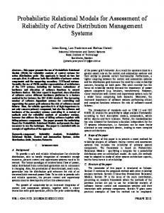
given polynomial function f of Z, are now derived. Here, the study is limited to the expected values of Z, 具Z典, and the second-order moments, 具ZZ典. In the literature, the system of mean field equations for 具Z典 and 具ZZ典 is often referred to as the Eulerian model or sometimes two-fluid model. As a matter of fact, the system of equations formed by the mean field equations should rather be called two-field model. Indeed, the spirit of the approach is to derive field equations for both phases by using arguments from statistical physics. Let us investigate how such equations are derived 共for incompressible turbulent flows carrying discrete particles of constant density but different diameters兲. Let us recall momentarily the Lagrangian and Eulerian tools that were defined in the previous section as well as the relations between them, see Fig. 1. A two-point fluid-particle Lagrangian PDF, p Lf p , 共extracted from the transitional PDF pˆ Lf p 兲 has been introduced and from it separate information on each phase was obtained in the form of the marginals p Lk . Associated MDFs (F Lk ) were defined and for both of them correspondence with the field 共Eulerian兲 description could be made 共this crucial step is indicated with dashed arrows in Fig. 1兲. It was then found that each Eulerian mass density function F Ek is propagated by the corresponding transitional PDF, pˆ Lk . The Fokker-Planck equations verified by F Ek can then be directly derived from the Fokker-Planck equations satisfied by the transitional PDFs pˆ Lk or from the FokkerPlanck equation verified by the transitional PDF pˆ Lf p . There is another, yet equivalent, way to go from the transitional PDF pˆ Lf p to the Eulerian MDFs F Ek , see Fig. 1. One can keep the joint 共one fluid point–one particle point兲 information by treating the two-point fluid-particle Eulerian MDF, F fEp . As indicated in Fig. 1, by direct integration, the Fokker-Planck equations verified by the marginals FkE can be obtained from the Fokker-Planck equation verified by FpEf which is, in its turn, obtained from the PDF verified by the transitional PDF pˆ Lf p . The latter equations are also verified by F Ek . To sum up, it is now known how the Fokker-Planck equations verified by the Eulerian MDFs F Ek can be derived. Let us show how mean field equations are obtained from the Fokker-Planck equations verified by F Ek . A. Fluid and discrete particle expectations

In the case of discrete particles of constant density but variable diameter carried by an incompressible fluid, all information is contained in the distribution functions p Ek (t,x;Vk , ␺k ) 关with ␺p ⫽(Vs , ␦ p ) for the discrete phase and ␺ f ⫽⭋ for the fluid兴. However, the definition of the expected values and the derivation of the mean field equations will be addressed, for both phase, in terms of the MDFs F Ek (t,x;Vk , ␺k )⫽ ␳ k p Ek (t,x;Vk , ␺k ) 共the reason for this will shortly be explained兲. The mathematical definition of the expected Eulerian value of a function H(Vk , ␺k ) 共a sufficiently smooth function attached to a given particle, i.e., a fluid or a discrete particle兲 is

␣ k 共 t,x兲具 ␳ k 典共 t,x兲具 Hk 典共 t,x兲 ⫽

冕

H共 Vk , ␺k 兲 F Ek 共 t,x;Vk , ␺k 兲 dVk d ␺k . 共37兲

Therefore, in the present formalism, all expected values must be understood as mass-weighted mean values. The fluctuating component of the variables attached to the discrete particles are, for the velocity of the discrete particles up ⫽Up ⫺ 具 Up 典 with 具 up 典 ⫽0, for the fluid velocity seen us ⫽Us ⫺ 具 Us 典 with 具 us 典 ⫽0, and for the diameter of the discrete particles d ⬘p ⫽d p ⫺ 具 d p 典 with 具 d ⬘p 典 ⫽0. Similarly, the fluctuating velocity for a fluid particle is given by u f ⫽U f ⫺ 具 Uf 典 . For the moments of the discrete phase, a general definition is introduced, that is a moment of order n⫹m⫹q 共with n⫹m⫹q⬎1兲,

␣ p 共 t,x兲 ␳ p 具共 d ⬘p 兲 n u s,i 1 ¯u s,i m u p, j 1 ¯u p, j q 典共 t,x兲 ⫽

冕

m

共 ␦ ⬘p 兲 n

兿

k⫽1

q

v s,i k

兿

l⫽1

v p, j l F Ep 共 t,x;Vp , ␺p 兲 dVp d ␺p ,

共38兲 where (i k , j l )苸兵 1,2,3 其 2 , ᭙(k,l). Different moments can then be obtained by choosing the appropriate values for 共n,m,q兲. In the present paper, information is limited to the second-order moments, i.e., n⫹m⫹q⫽2. At last, the moments of order n for the fluid phase are given by

冕兿 n

␣ f 共 t,x兲 ␳ f 具 u f ,i 1 ¯u f ,i n 典共 t,x兲 ⫽

k⫽1

v f ,i k F Ef 共 t,x;V f 兲 dV f .

共39兲

All second-order moments are listed in Table I. Note that the dimension of the space associated to these moments is already 34, and this gives a foretaste, first, of the level of complexity when one formulates mean field equations for polydispersed turbulent two-phase flows, and second, of the amount of computational effort needed to solve such a system of equations 共when it is finally closed兲. It is now necessary to clarify the correspondence between the mathematical expectations, Eq. 共37兲, and Monte Carlo estimations drawn from a finite ensemble of particles. With Eq. 共15兲 and by approximating ␦ (xk ⫺yk ) as 1/␦ Vx where ␦ Vx is a small-volume around point xk , it is straightforward to write Eq. 共37兲 as N

k

1 x i ␣ k 共 t,x兲具 ␳ k 典共 t,x兲具 Hk 典 ⯝ m H„Uik 共 t 兲 , ␾ ik 共 t 兲 …. ␦ Vx i⫽1 k

兺

共40兲

Here N kx is the number of fluid (k⫽ f ) or discrete (k⫽p) particles in volume ␦ Vx and m ik is the mass of a fluid or discrete particle indexed i. The preceding equation can be written by supposing that 共i兲 all particles in ␦ Vx represent different realizations, 共ii兲 space homogeneity is fulfilled in ␦ Vx , and 共iii兲 N kx is sufficiently large so that the ensemble

046301-8



FIG. 1. Derivation of the mean field equations from the two-point fluid-particle Eulerian mass density function 共→兲 or derivation of the mean field equations from the marginal Lagrangian PDFs 共⇒兲. The Eulerian approach corresponds to the field equations whereas the Lagrangian approach is indicated by the symbol 关*兴

⳵ ⳵ 共 ␣ ␳ 具H 典兲⫹ 共 ␣ ␳ 具V H 典兲 ⳵t f f f ⳵ x i f f f ,i f

average is a good estimation of the mathematical expectation. Furthermore, by making the following approximation N

k

1 x i ␣ k 共 t,x兲具 ␳ k 典共 t,x兲 ⯝ m , ␦ Vx i⫽1 k

兺

⫽␣ f␳

共41兲

⫹

one has k

具 Hk 典 ⯝ 兺

i⫽1

冒兺 k

Nx

Nx

m ik H„Uik 共 t 兲 , ␾ ik 共 t 兲 …

i⫽1

m ik ,

共42兲

which is indeed the discrete form of the Eulerian massweighted mean value of a given function. In the particular case of an incompressible fluid, since fluid particles have then a constant mass, the preceding expression is of course simplified to yield the local ensemble average. For discrete particles of constant density such a simplification is not relevant. Indeed, such particles may have different diameters and therefore different masses. The natural averaging operator is therefore the mass-weighted average.

冕

冔

冓

共 A p→ f ,i 兩 x,V f 兲

⳵ Hf E F 共 t,x;V f 兲 dV f . ⳵V f f

⳵ ⳵ 共 ␣ ␳ 兲⫹ 共 ␣ ␳ 具 U 典兲 ⫽0, ⳵t f f ⳵ x i f f f ,i

␣f␳ f

冔共44兲

共45兲

Df ⳵ 共 ␣ ␳ 具 u u 典兲 ⫹ ␣ f ␳ f 具 A f ,i 典 ⫹I M 具 U f ,i 典 ⫽⫺ f ,i Dt ⳵ x j f f f ,i f , j 共46兲

and after some algebra, the Reynolds-stress equations are given by

␣f␳f

⳵ F Ef ⳵ F Ef ⳵ ⫽⫺ ⫹V f ,i 共A FE兲 ⳵t ⳵xi ⳵ V f ,i f ,i f ⳵2 1 ⫹ 共关 B j B Tf 兴 i j F Ef 兲 2 ⳵ V f ,i ⳵ V f , j ⳵ ⫺ 共具 A p→ f ,i 兩 x,V f 典 F Ef 兲 , ⳵ V f ,i

冓

⳵ Hf ⳵ 2 Hf 1 ⫹ ␣ f ␳ f 共 B f B Tf 兲 i j ⳵ V f ,i 2 ⳵ V f ,i ⳵ V f , j

In this derivation, it has been supposed that A f , B f , and H f are sufficiently smooth so that all generalized integrals converge 共by construction, F Ef and ⳵ F Ef / ⳵ V f ,i converge to zero when, at least, one component of the fluid velocity goes to infinity, V f ,i →⫾⬁兲. By replacing H f by H f ⫽1, H f ⫽V f ,i and H f ⫽V f ,i V f , j , the continuity equation the momentum equations 共mean field equations for U f 兲, and the Reynoldsstress equations 共mean field equations for 具 u f u f 典兲 are obtained, respectively. The Reynolds-stress equations can also be derived using another route, i.e., by making a change of coordinates in sample space 共this procedure will be outlined in the next section兲. The continuity and momentum equations are

B. Mean field equations for the fluid phase

In order to obtain the mean field equations for the mean fluid velocity 具 U f ,i 典 and the second-order velocity moment 具 u f ,i u f , j 典 , a standard procedure is used in analogy with the derivations that can be found in kinetic theory 关22,23兴. This procedure is general and can be followed to obtain the mean field equations verified by any moment. The expected value of a function H f (V f ) is defined by Eq. 共37兲共␺ f is omitted since the flow is incompressible兲. With Eqs. 共23兲 and 共36兲, and the explanations of Fig. 1, it is straightforward to write the Fokker-Planck equation verified by F Ef (t,x;V f ),

f

A f ,i

Df ⳵ 共 ␣ ␳ 具u u u 典兲具 u f ,i u f , j 典 ⫽⫺ Dt ⳵ x k f f f ,i f , j f ;k ⫺ ␣ f ␳ f 具 u f ,i u f ,k 典

⳵具U f , j典 ⳵xk

⫺ ␣ f ␳ f 具 u f , j u f ,k 典

⳵ 具 U f ,i 典 ⳵xk

⫹ ␣ f ␳ f 具 A f ,i v f , j ⫹A f , j v f ,i 典 ⫹ ␣ f ␳ f 具共 B f B Tf 兲 i j 典 ⫹I Rf ,i j ,

共43兲

and if one multiplies Eq. 共43兲 by H f and applies the 具 • 典 operator, one can write after some algebra

共47兲

where the Eulerian derivative along the path of a fluid particle is denoted D f /Dt with D f /Dt⫽ ⳵ / ⳵ t⫹ 具 U f ,m 典 ⳵ / ⳵ x m . In both the momentum and Reynolds-stress equations, there is a

046301-9



TABLE I. Definition of the second-order moments: all moments attached to the discrete particles are calculated with Eq. 共38兲 whereas the Reynolds stresses are obtained from Eq. 共39兲. Second-order moment

n

m

p

Variable

Reynolds stresses Second-order particle velocity moment Second-order fluid velocity seen moment Fluid-particle velocity correlation tensor Diameter-particle velocity correlation tensor Diameter-fluid velocity seen correlation tensor Second-order diameter moment

2 0 0 0 1 1 2

0 2 1 0 1 0

2 0 1 1 0 0

具 u f ,i u f , j 典具 u p,i u p, j 典具 u s,i u s, j 典具 u p,i u s, j 典具 d ⬘p u p,i 典具 d ⬘p u s,i 典具 (d ⬘p ) 2 典

R term 共I M f ,i for the momentum equations and I f ,i j for the Reynolds-stress equations兲 that accounts for the influence of the discrete particles on the fluid phase. For both terms, further considerations are necessary before their final form can be obtained. Let us start with I M f ,i . The term I M f ,i is expressed as a function of the conditional expectation of a random variable 共as it has been suggested in Sec. III D 4兲

␣p IM f ,i ⫽ ␣f

冕具

⌸ p,i 兩 V f 典 F Ef 共 t,x;V f 兲 dV f ,

冕

⌼ p,i p 共 ⌼p 兩 V f 兲 F Ef 共 t,x;V f 兲 dV f d⌼p .

冉冊

␣p ␣ ␳ 具 ⌸ p,i 典 ⫽⫺ ␣ p ␳ p 具 A Dp,i 典 . ␣f f f

共50兲

The term I Rf ,i j that enters the Reynolds-stress equations is expressed by M I Rf ,i j ⫽ 共 I Ef ,i j ⫹I Ef , ji 兲 ⫺ 共具 U f ,i 典 I M f , j ⫹ 具 U f , j 典 I f ,i 兲 ,

共51兲

where I Ef ,i j ⫽

冕具

I Rf ,i j

A p→ f ,i 兩 x,V f 典 V f , j F Ef 共 t,x;V f 兲 dV f .

I Ef ,i j ⫽

冉冊冕 ␣p ␣␳ ␣f f f

⌼ p,i V f , j p 共 ⌼ p,i ,V f 兲 dV f d⌼p

共53兲

that is, I Ef ,i j ⫽⫺ ␣ p ␳ p 具 A Dp,i U s, j 典 ,

共54兲

and finally

共49兲

Let us introduce the joint PDF of ⌸p and U f , p(⌼p ,V f ), and the definition of the conditional PDF p(⌼p ,V f ) ⫽p(⌼ p,i 兩 V f )p(V f ), where p(V f ) denotes the normalized PDF of U f at location x. From the relations given in Sec. III C 2 one has directly ␣ f ␳ f p(V f )⫽F Ef (t,x;V f ) and therefore the term I M f ,i can be written as IM f ,i ⫽

symbolizes Eq. 共46兲. Using the same reasoning as in the case of the momentum equation and applying the model of Sec. III D 4 and the results of Sec. III C 2, the term I Ef ,i j is expressed as

共48兲

where the ratio ␣ p / ␣ f expresses the probability to have a random force conditioned on the fact that there is a fluid particle at x. Let ⌼p be the sample-space value for the random variable ⌸p at time t and location x. It is then possible to rewrite the previous equation as 关where p(⌼p 兩 V f ) is the PDF of ⌸p conditioned upon U f 兴

␣p IM f ,i ⫽ ␣f

具 U f ,i 典 N( 具 U f , j 典 )⫹ 具 U f , j 典 N( 具 U f ,i 典 )⫽0, where the operator N

I Rf ,i j ⫽⫺ ␣ p ␳ p 具 A Dp,i u s, j ⫹A Dp, j u s,i 典 ⫹ ␣ p ␳ p 共 Ud,i 具 A Dp, j 典 ⫹Ud, j 具 A Dp,i 典兲 .

共55兲

The expression of I Rf ,i j is written in a form where the difference 具 U f , j 典 ⫺ 具 U s, j 典 , denoted Ud,i , explicitly appears. This quantity represents, at a given time t and a given location x, the difference between the expected fluid velocity and the expected fluid velocity seen by the discrete particles. Finally, in Table II, a list of the terms to be closed is given. A distinction is made between the unclosed terms and the third-order moments that appear naturally in the PDE verified by 具 u f u f 典 . The closure issue will be addressed in Sec. VI where a closed two-field model is derived. TABLE II. List of the unknown terms in the mean field equations of the continuous phase.

共52兲

This form of is easily found as follows: the PDE, which is written for the local instantaneous second-order moment 具 U f ,i U f , j 典 , is linearly combined with the PDE for 具 U f ,i 典具 U f , j 典 . The latter PDE is obtained by developing

Equation Eq. 共46兲 Eq. 共47兲

046301-10

Variable

具U f典

具 u f ,i u f , j 典

Unclosed term IM p f ,i 具 A f ,i 典 ,u f , j 典具 (B f B Tf ) i j 典

I Rp f ,i j 具 A f

Third-order moment

具 u f ,i u f , j u f ,k 典



C. Mean field equations for the discrete phase

The mean field equations for the discrete phase are now obtained following the procedure presented in Sec. IV B when deriving mean field equations for the fluid phase. The expectation of a given function Hp (Vp , ␺p ) is defined by Eq. 共37兲. Using Eqs. 共23兲 and 共36兲, and the explanations of Fig. 1, it is straightforward to prove that F Ep (t,x;Vp , ␺p ) verifies the following Fokker-Planck equation:

⳵ F Ep ⳵ F Ep ⳵ ⳵ ⫹V p,i ⫽⫺ 共 A FE兲⫺ 共A FE兲 ⳵t ⳵xi ⳵ V p,i p,i p ⳵ V s,i s,i p ⫹

⳵2 1 关共 B s B sT 兲 i j F Ep 兴 2 ⳵ V s,i ⳵ V s, j

⫺

⳵ 共具 A p→s,i 兩 x,Vp , ␺p 典 F Ep 兲 . 共56兲 ⳵ V s,i

As it was done in the previous section, Eq. 共56兲 is multiplied by Hp and the 具 • 典 operator is applied. Then, as done in Sec. IV B, As , Ap , Bs , and Hp are assumed to be sufficiently smooth so that all generalized integrals converge 共F Ep , ⳵ F Ep / ⳵ V s,i , and ⳵ F Ep / ⳵ V p,i converge to zero when, at least, one component of Vs or Vp goes to infinity兲. After some derivations, one can write

⳵ ⳵ 共 ␣ ␳ 具H 典兲⫹ 共 ␣ ␳ 具V H 典兲 ⳵t p p p ⳵ x i p p p,i p

冓

⫽ ␣ p ␳ p A p,i

冔

冓

⳵ Hp ⳵ Hp ⫹ ␣ p ␳ p A s,i ⳵ V p,i ⳵ V s,i

冓

⳵ 2 Hp 1 ⫹ ␣ p ␳ p 共 B s B sT 兲 i j 2 ⳵ V s,i ⳵ V s, j ⫹

冕具

A p→s,i 兩 x,Vp , ␺p 典

冔

冔

␣ p␳ p

Dp ⳵ 具 d p 典 ⫽⫺ 共 ␣ p ␳ p 具 d ⬘p u p,i 典兲 , Dt ⳵x

where ␹ ⫽( ␣ p ␳ p )/( ␣ f ␳ f ) and where the Eulerian derivative along the path of a discrete particle is denoted D p /Dt with D p /Dt⫽ ⳵ / ⳵ t⫹ 具 U p,m 典 ⳵ / ⳵ x m . The mean field equations verified by the second-order moments 关n⫹m⫹q⫽2 in Eq. 共38兲兴 can be derived in a way that requires less algebra than the procedure that has been outlined so far by using Eq. 共57兲 and the right function for Hp . By introducing a change of coordinates in sample space, v⫽V⫺ 具 U典 (t,x) and ␦ ⬘p ⫽ ␦ p ⫺ 具 d p 典 (t,x) 共where v stands for vp or vs 兲, it is straightforward to write the Fokker-Planck equation verified by F Ep (t,x;vp ,vs , ␦ ⬘p ). Then using the usual technique, the PDE verified by a given function Hp (vp ,vs , ␦ p ) is derived in the same fashion as for Eq. 共57兲 where similar conditions for the convergence of the generalized integrals are required. This procedure is not detailed here but it can be found with all necessary derivations in Ref. 关12兴. After some algebra, one finds for 具 u p,i u p, j 典 ,

␣ p␳ p

Dp ⳵ 共 ␣ ␳ 具u u u 典兲具 u u 典 ⫽⫺ Dt p,i p, j ⳵ x k p p p,i p, j p,k

␣ p␳ p

The PDEs for the specified discrete particle expectations can now be derived, simply by choosing the right function for Hp . Hp ⫽1,V p,i ,V s,i , ␦ p gives the continuity equation, the momentum equation, the PDE verified by the expected fluid velocity seen, and the PDE for the mean diameter, respectively. These equations have the form

⳵ 具 U p,i 典 ⳵xk

Dp ⳵ 共 ␣ ␳ 具u u u 典兲具 u s,i u p, j 典 ⫽⫺ Dt ⳵ x k p p s,i p, j p,k

共58a兲

⫺ ␣ p ␳ p 具 u s,i u p,k 典

⳵ 具 U p, j 典 ⳵xk

⫺ ␣ p ␳ p 具 u p, j u p,k 典

⳵ 具 U s,i 典 ⳵xk

⫺ ␣ p ␳ p ␹ 具 A Dp,i u p, j 典 ,

␣ p␳ p

Dp 具u u 典 Dt s,i s, j

⫽⫺

⳵ ⳵ 具 U s, j 典 ( ␣ ␳ 具 u u u 典 )⫺ ␣ p ␳ p 具 u s,i u s,k 典 ⳵ x k p p s,i s, j s,k ⳵xk

⫺ ␣ p ␳ p 具 u s, j u s,k 典

⳵ 具 U s,i 典 ⫹ ␣ p ␳ p 具 A s, j v s,i ⫹A s,i v s, j 典 ⳵xk

⫹ ␣ p ␳ p 具共 B s B sT 兲 i j 典 ⫺ ␣ p ␳ p ␹ 具 A Dp, j u s,i ⫹A Dp,i u s, j 典 .

共58c兲

共60兲

and for 具 u s,i u s, j 典 ,

Dp ⳵ 共 ␣ ␳ 具 u u 典兲 ⫹ ␣ p ␳ p 具 A s,i 典具 U s,i 典 ⫽⫺ Dt ⳵ x j p p s,i p, j ⫺ ␣ p ␳ p ␹ 具 A Dp,i 典 ,

⫺ ␣ p ␳ p 具 u p, j u p,k 典

⫹ ␣ p ␳ p 具 A s,i v p, j 典 ⫹ ␣ p ␳ p 具 A p, j v s,i 典

Dp ⳵ 共 ␣ ␳ 具 u u 典兲 ⫹ ␣ p ␳ p 具 A p,i 典 , 具 U p,i 典 ⫽⫺ Dt ⳵ x j p p p,i p, j 共58b兲

␣ p␳ p

⳵ 具 U p, j 典 ⳵xk

for 具 u p,i u s, j 典 ,

共57兲

␣ p␳ p

⫺ ␣ p ␳ p 具 u p,i u p,k 典

⫹ ␣ p ␳ p 具 A p,i v p, j ⫹A p, j v p,i 典 , 共59兲

⳵ Hp E F 共 t,x;Vp , ␺p 兲 dVp d ␺p . ⳵ V s,i p

⳵ ⳵ 共 ␣ ␳ 兲⫹ 共 ␣ ␳ 具 U 典兲 ⫽0, ⳵t p p ⳵ x i p p p,i

共58d兲

After some calculus, one finds for 具 d ⬘p u p,i 典 ,

046301-11

共61兲


␣ p␳ p


Dp ⳵ 共 ␣ ␳ 具d ⬘u u 典兲具 d ⬘p u p,i 典 ⫽⫺ Dt ⳵ x j p p p p,i p, j ⫺ ␣ p ␳ p 具 d ⬘p u p, j 典

V. MEAN FIELD–PDF APPROACH

⳵ 具 U p,i 典 ⳵x j

⫺ ␣ p ␳ p 具 u p,i u p, j 典

⳵ 具 d p典 ⫹ ␣ p ␳ p 具 A p,i d ⬘p 典 , ⳵x j 共62兲

for 具 d ⬘p u s,i 典 ,

␣ p␳ p

Dp ⳵ 共 ␣ ␳ 具d ⬘u u 典兲具 d ⬘p u s,i 典 ⫽⫺ Dt ⳵ x j p p p s,i p, j ⫺ ␣ p ␳ p 具 d ⬘p u p, j 典

⳵ 具 U s,i 典 ⳵x j

⫺ ␣ p ␳ p 具 u s,i u p, j 典

⳵ 具 d p典 ⫹ ␣ p ␳ p 具 A s,i d ⬘p 典 ⳵x j

⫺ ␣ p ␳ p ␹ 具 A Dp,i d ⬘p 典 ,

共63兲

and for 具 (d ⬘p ) 2 典 ,

␣ p␳ p

Dp ⳵ „␣ ␳ 具共 d ⬘ 兲 2 u 典 … 具共 d ⬘p 兲 2 兲典 ⫽⫺ Dt ⳵ x i p p p p,i ⫺2 ␣ p ␳ p 具 d ⬘p u p,i 典

⳵ 具 d p典 , ⳵xi

共64兲

which concludes the set of mean field equations for the second-order moments related to the discrete phase. A first glance at the amount of terms that are unknown, not to mention the third-order moments, gives an insight into the intricate work which is left, that is to provide suitable closures in order to use the model in practical computations. Table III gives a list of all unknown terms that appear in the mean field equations for the discrete phase. This information has to be supplemented by Table II to obtain the total amount of unknown terms. The wise reader has already realized that a tremendous work is waiting and it is already clear that such an approach 共mean field equations兲 can only be used in practice when further contractions are possible 共the dimension of the system is 46 with 19 unknown terms, which is nearly intractable兲, that is in a simplified case. This is the subject of Sec. VI where an example of a practical model is given in the case where there is no size distribution for the discrete particles, i.e., the particle diameter is eliminated from the state vector. As mentioned in the Introduction, there are alternatives to the mean field equations, for example, the Lagrangian approach. It is now shown that, with the Lagrangian approach, a great deal of the difficulties, created by the treatment of the discrete phase with mean field equations, can be eliminated.

In the previous section, the derivation of the mean field equations 共up to the second-order moments兲 for both phases has been presented. It has been explained, in both Tables II and III, that apart from the third-order moments, writing mean field equations is a move that generates, from a closed mesoscopic model, unclosed terms at the macroscopic level. Indeed, one has to express the expectations of complex nonlinear expressions of the basic variables, for example, terms D such as 具 A D i 典 or 具 A i u s,i 典 . There is a natural way to avoid most of these difficulties, which is the Lagrangian approach. In fact, in such an approach, mean field equations are used solely for the fluid phase whereas for the discrete phase information is still available at the mescocopic level, see Fig. 1. Actually, the term ‘‘Lagrangian approach’’ is rather misleading. Here the approach is called from now on mean field–PDF approach since mean fields are used for the description of the fluid and a PDF is employed for the discrete phase. It is now clear that such a method contains the mean field approach. Although the description of the fluid is identical for the two-field model and the mean field–PDF model, the treatment of the discrete phase is different. In the mean field–PDF approach, information is available for the local instantaneous values of any variable attached to the discrete phase whereas in the two-field approach a contraction has been made 共only the two first moments of the variables of interest are available兲. This distinction is apparently often missed in the literature. The two models are frequently compared without specifying that they do not correspond to the same level of information. As a matter of fact, if such a comparison is attempted, one should not only look at the computational effort and the easiness of implementation but also at the information that can be extracted from the model. If one is interested in, for instance, discrete-particle residence time or conditional statistics, the mean field–PDF approach can provide such information but the two-field model cannot. The mean field–PDF model equations are, for the fluid, Eqs. 共45兲 to 共47兲, and for the particles Eqs. 共30兲. The closure problem has been greatly simplified since the exhaustive list of Table III disappears. Closure is now limited to Table II. VI. PRESENTATION AND HIERARCHY OF PRACTICAL MODELS

So far, a probabilistic approach to polydispersed turbulent two-phase flows has been presented. From it, mean field equations have been written for the expectations and the second-order moments of the variables that form the state vector Z. The SDEs, proposed for the trajectories of Z, and the mean field equations, derived for 具Z典 and 具ZZ典, are limited to the case of nonreacting turbulent polydispersed twophase flows where the fluid is incompressible and the particles are noncolliding hard spheres. Yet, the mean field equations, to be used in practical simulations, present an intricate challenge: the dimension of the problem is very large and the amount of information that has to be closed is far from being negligible. It is possible, however, in practice, to use the mean field equations for computations if further as-

046301-12



TABLE III. List of the unknown terms in the mean field equations of the discrete phase. Equation Eq. Eq. Eq. Eq. Eq. Eq. Eq. Eq. Eq.

共58b兲共58c兲共58d兲共59兲共61兲共60兲共62兲共63兲共64兲

Variable

Unclosed term

具 U p典具 U s典具 d p典

具 A p,i 典具 A Dp,i 典具 A s,i 典

具 u p,i u p, j 典具 u s,i u s, j 典具 u s,i u p, j 典具 d ⬘p u p,i 典具 d ⬘p u s,i 典具 (d ⬘p ) 2 典

具 A p,i u p, j 典具 A s, j u s,i 典具 A Dp,i u s, j 典具 (B s B sT ) i j 典具 A p, j u s,i 典具 A s, j u p,i 典具 A Dp, j u p,i 典具 A p,i d ⬘p 典具 A s,i d ⬘p 典

sumptions are made on the nature of the flow, i.e., if further contractions are made 关24兴. Before presenting the form of the mean field equations that are used in simulations, let us show an example of a two-point PDF model from which practical Lagrangian and Eulerian models can be extracted. The presentation follows the hierarchy of models that has been displayed in the previous sections: 共i兲 a two-point PDF model where information is available at the mesoscopic level for both phases, 共ii兲 a mean-field–PDF model where a first contraction is made for the fluid and 共iii兲 a two-field model where further contraction is performed 共information is given solely for the two first moments of both phases兲.

A. Example of a two-point PDF model

From now on, the external force field FE is reduced to gravity g. In the single-phase flow case, one can use the RSM 共Reynolds-stress model兲 equations since there is a direct connection between a Langevin equation and a RSM equation 关10兴. However, another route can be chosen using arguments from statistical physics 关25兴. The model is given by A f ,i ⫽⫺

1 ⳵具 P典 U f ,i ⫺ 具 U f ,i 典 ⫹g i ⫺ ⫹G ai j 共 U f , j ⫺ 具 U f , j 典兲 , ␳ f ⳵xi TL 共65兲 B f ,i j ⫽ 冑C 0 具 ⑀ 典 ␦ i j ,

Third-order moment

共66兲

where 具 P 典 (t,x f ) is the mean pressure field and 具 ⑀ 典 (t,x f ) represents the mean dissipation rate of turbulent kinetic energy, 2k f ⫽ 具 u2f 典 (t,x f ). T L is the fluid integral Lagrangian time scale, i.e., T L ⫽Ck f / 具 ⑀ 典 , where 1/C⫽1/2⫹3C 0 /4 and C 0 is a constant 共given by Kolmogorov theory兲. G ai j is an anisotropy matrix 共whose precise form is not important here兲 that depends solely on the moments of Z f . The construction of the SDE for the simulation of the time increments of the fluid velocity seen is an open question 关12,21兴 and the form that is proposed here belongs to a set of possible solutions. The present model is expressed by 关12兴

A s,i ⫽⫺

具 u p,i u p, j u p,k 典具 u s,i u s, j u s,k 典具 u s,i u p, j u p,k 典具 d ⬘p u p,i u p, j 典具 d ⬘p u s,i u p, j 典具 (d ⬘p ) 2 u p,i 典

1 ⳵具 P典 ⫹g i ⫺G i j 共 U s, j ⫺ 具 U s, j 典兲 ⫹ 共具 U p, j 典 ␳ f ⳵xi

⫺ 具 U s, j 典兲

⳵ 具 U f ,i 典 , ⳵x j

冋

2 ⫽ 具 ⑀ 典 C 0b i B s,ii

共67兲

冉

˜k f 2 ˜k f ⫹ b i ⫺1 kf 3 kf

冊册

,

共68兲

where B s,i j is expressed in its simplest form 共as a diagonal and nonisotropic matrix兲 and G i j is given by G i j * . T L,i * is the fluid integral Lagrangian time scale ⫽ ␦ i j /T L,i sampled along the trajectories of the discrete particles. This time scale can be evaluated by a formula due to Csanady 关26兴 as 共if gravity is aligned with the first coordinate labeled 1兲

* ⫽T L T L,i

冒冉

1⫹Ci

兩具 Ur 典兩 2 2k f /3

冊

1/2

,

共69兲

where C 1 ⫽ ␤ 2 , C 2 ⫽C 3 ⫽4 ␤ 2 and ␤ is the ratio of the fluid Lagrangian and Eulerian integral time scales, ␤ ⫽T L /T E . The formula of Csanady implies that, even in the simplest case, G i j is a nonisotropic diagonal matrix. To complete the definition of Eq. 共68兲, 3

2 3

˜k f ⫽

兺

i⫽1

冒兺 3

b i 具 u 2i 典

i⫽1

bi ,

共70兲

* . In practice, the PDF approach given by where b i ⫽T L /T L,i Eqs. 共31兲 is not self-sufficient since one has to compute the mean pressure field 具 P 典 (t,x f ) and the mean dissipation of turbulent kinetic energy, 具 ⑀ 典 (t,x f ). It is possible, following a procedure outlined by Pope 关9兴, to derive for each phase a Poisson equation verified by the mean pressure. This Poisson equation, for each phase, guarantees that the continuity equation of each phase is satisfied. The sum of both equations is a Poisson equation that expresses the mass conservation of the mixture. For 具⑀典, a model, based on Kolmogorov’s third hypothesis 关ln(⑀) is normally distributed in homogeneous turbulence兴, has been developed 关27兴. It consists in writing a Langevin equation for the frequency rate ␻ ⫽ ⑀ /k f along the trajectories of the fluid particles,

046301-13


d ␻ ⫽ 关 A ␻ ⫹A ␻p→ f 兴 dt⫹B ␻ dW,


共71兲

where the drift and diffusion coefficients, A ␻ and B ␻ respectively, are specified in Ref. 关27兴. The new state vector becomes Z⫽(Z f ,Zp , ␻ ) and A ␻ and B ␻ are functions of t, Z and its moments. Equation 共71兲 has been supplemented by a term A ␻p→ f accounting for the influence of the particles on the local instantaneous frequency. A possible model for this term reads A ␻p→ f ⫽G ␻ ⌸p,i V f ,i ,

共72兲

which means that the influence of the particles on ␻ is related to the local instantaneous work performed by the action of the particles on the fluid multiplied by a coefficient that is a function of the moments of Z only. This subject is not dwelt upon here and only the reduced state vector Z ⫽(Z f ,Zp ) is under investigation. For the complete state vector, the Fokker-Planck equation, Eq. 共36兲, can easily be extended by adding the additional terms generated by the additional dimension 共␻兲. We do not dwell upon the different models that can be derived for the drift vectors and the diffusion matrices and we try instead to retain the main features that are of importance for the derivation of the mean field equations. Detailed discussions and proofs of the modeling choices can be found in Ref. 关12兴. B. Derivation of a practical mean field-PDF model

In the case of the fluid, the only difficulty 共if one accepts a gradient hypothesis for the third-order moments兲 when writing mean field equations is the coupling terms both in the momentum equations and the RSM equations. In the case of the discrete phase, a closed mesoscopic model, in the form of Langevin equations, has already been provided, Eqs. 共67兲 and 共68兲. When the PDEs for the fluid are solved by classical methods 共for example, finite volume methods兲 the coupling terms in a computational cell can then be calculated in a natural way by making the classical hypotheses, 共i兲 homogeneity in space, and 共ii兲 the approximation of the expectation by ensemble averaging when the number of samples in the cell is sufficient. For example, for the coupling term in the momentum equations, let V f be the volume of the computational cell that contains N p discrete particles. The total force in the cell due to the N p particles is 共with N p large enough兲

same procedure can be applied to the coupling term in the RSM equations, 具 F p→ f ,i U f , j 典 . The level of simplicity of the mean field-PDF model 共in comparison to the simplified two-field model that is going to be presented in Sec. VI C兲 and its ability to compute complicated terms in the polydispersed case are noteworthy. It is a school example of the reason why PDF approaches should be preferred to mean field approaches in cases where the physics of the flow becomes complex. Examples of practical computations performed with the mean field-PDF approach can be found in Ref. 关12兴. C. Derivation of a practical two-field model

The derivation of the model is treated in two different steps. First, a list of hypotheses that make it possible to reduce the dimension d of the system is given and second, it is shown how to close the n unclosed terms by making further hypotheses. It is recalled that, in the frame of our study that is limited to second-order moments, d⫽46 and n⫽12 关seven third-order moments and now five unclosed terms, the other ones can be directly closed, see Eqs. 共65兲–共70兲 and Tables II and III兴. 1. Reduction of the dimension of the system

All hypotheses needed to reduce the dimension of the original system are now given. 共i兲 Let us consider the case where the distribution in diameter of the discrete particles is ‘‘narrow’’ enough so that the statistics involving the diameter can roughly be approximated as constant in time and space 共this hypothesis is equivalent to state that the suspension is monodispersed and therefore segregation effects cannot be quantified anymore兲. The sample space is only reduced by one dimension but eight PDEs have already been eliminated 共all PDEs involving the particle diameter兲, that is the new dimension of the system is d⫽38. 共ii兲 Furthermore, it is assumed that there is no statistical bias between the statistics of the second-order moments for the fluid velocity seen and for the fluid velocity, i.e., 具 us us 典 ⯝ 具 uf uf 典 . So far, with two hypotheses, which severely limit the number of problems which can be treated, the dimension of the problem has been reduced to d⫽32 but many unclosed terms remain n⫽9 共four third-order moments and five unclosed terms兲. 2. Treatment of the unclosed terms

Np

Fp→ f ⫽

兺

n⫽1

␳ p Vpn AD,n p ,

共73兲

where Vpn is the volume of the discrete particle labeled n. The previous equation is indeed the mean momentum exNp Vpn )/V f 兴 change 关using ␣ p ⯝( 兺 n⫽1

具 Fp→ f 典 ⫽ ␣ p ␳ p V f 具 ADp 典 .

共74兲

One can, therefore, see that complicated nonlinear terms such as 具 ADp 典 are computed in a simple and natural way. The

Let us now enumerate the hypotheses that are necessary to make in order to treat the unclosed terms 共the hypotheses are numbered in continuation with the previous subsection and this for the sake of clarity兲. 共iii兲 It is assumed that all third-order tensors 具 Z i Z j Z k 典 can be expressed as a function of what is known 共or solved for兲, that is, 具 Z i 典 and 具 Z i Z j 典共a macroscopic closure is made with all the difficulties and the risks that such a move entails兲. This is done in analogy with classical turbulence results where one seeks macroscopic relations of the type 共k is the phase index兲

046301-14


⫺ 具 u k,i u k, j u k,m 典 ⫽D k,mn 共具 Z典 , 具 ZZ典兲

⳵ 具u u 典, ⳵ x n k,i k, j


I k,i ⫽Ik 共75兲

and ⫺ 具 u s,i u p, j u p,m 典 ⫽D sp,mn 共具 Z典 , 具 ZZ典兲

⳵ 具u u 典, ⳵ x n s,i p, j

共76兲

where D k,i j and D sp,i j are often called ‘‘turbulent diffusion tensors.’’ Their possible forms are not given here but can be found, for example, in Ref. 关28兴. 共iv兲 It is assumed that, for heavy particles, a good approximation of Ap is 关Eq. 共28兲 is supplemented with the mean pressure gradient兴 A p,i ⫽⫺

1 ⳵具 P典 ⫹A Dp,i ⫹g i , ␳p ⳵xi

共77兲

where ADp is defined by Eq. 共32兲. In this expression, the influence of pressure fluctuations has explicitly been neglected. Indeed, the pressure that should be involved in the gradient is the local instantaneous pressure seen, P s „t,x p (t)…, along the path of the discrete particle, which is different from the pressure field P„t,x f (t)… seen around the fluid particles. Therefore, it has been assumed that the field P s ⫺ 具 P 典 has no influence on the motion of the discrete particles. 共v兲 Let us suppose that all terms involving ADp can be linearized as follows 共where, in our case, G(u) is a linear function of u⫽1,us ,up 兲:

具 ADp G共 u兲典 ⫽

1 具共 Us ⫺Up 兲 G共 u兲典 , 具 ␶ p典

具 ␶ p 典 ⫽ ␶ p 共具 Z典 , 具 ZZ典兲 .

共78兲共79兲

This final assumption allows us to close all terms involving ADp and more generally Ap . After a subsequent number of hypotheses, it now possible to finalize our task and give a simplified, but still quite intricate (d⫽32), closed two-field model.

␣ p␳ p 共具 U s,i 典 ⫺ 具 U p,i 典兲 . 具 ␶ p典

Here, Ik is equal to 1 if k⫽p and to ⫺1 if k⫽ f . Bearing in mind the models presented above and hypotheses 共iii兲–共v兲, the remaining equations can now be written. For the expectation of the fluid velocity seen, 具 Us 典 , it is found that the sum of the terms to close read 关the two last terms on the righthand side of Eq. 共58c兲兴

冋

␣ p␳ p ⫺

册

⳵ 具 U f ,i 典 1 ⳵具 P典 ⫹g i ⫹ 共具 U p, j 典 ⫺ 具 U s, j 典兲 ⫺ ␹ I p,i , ␳ f ⳵xi ⳵x j 共82兲

where, as mentioned before, ␹ ⫽ ␣ p ␳ p / ␣ f ␳ f . For the RSM equations, as done for the expected fluid velocity seen, only the sum of the terms to close is given, and this for the sake of clarity. The closure of the third-order moments is immediate by resorting to hypothesis 共iii兲. Using hypothesis 共ii兲, the sum of the three last terms on the right-hand side of Eq. 共59兲 is ⫺

␣f␳f 关具 u f ,i u f , j 典 ⫺ 32 k f ␦ i j 兴 ⫹ ␣ f ␳ f 关 G aik 具 u f , j u f ,k 典 T

⫹G ajk 具 u j,i u f ,k 典兴 ⫹

␣ p␳ p 关 ⫺2 具 u f ,i u f , j 典 ⫹M i j ⫹Ud,i 具 U r, j 典具 ␶ p典

⫹Ud, j 具 U r,i 典兴 ⫺ ␣ f ␳ f 32 具 ⑀ 典 ␦ i j ,

␣ k␳ k

Dk ⳵具 P典 ⳵ ⫺ 共 ␣ ␳ 具 u u 典兲 ⫹I k,i 具 U k,i 典 ⫽⫺ ␣ k Dt ⳵xi ⳵ x j k k k,i k, j ⫹ ␣ k␳ kg i ,

␣ p ␳ p 具 A p,i u p, j ⫹A p, j u p,i 典 ⫽⫺

␣ p␳ p 关 2 具 u p,i u p, j 典 ⫺M i j 兴 , 具 ␶ p典共84兲

and for the fluid-particle velocity moment, the sum of the three last terms on the right-hand side of Eq. 共60兲 is

␣ p␳ p 关具 u f ,i u f , j 典 ⫺ 共 1⫹ ␹ 兲具 u s,i u p, j 典 ⫹ ␹ 具 u p,i u p, j 典兴具 ␶ p典

共80兲

where the interaction term l k,i is simply given by linearization of ADp as explained in hypothesis 共v兲共the precise form of the calculation of 具 ␶ p 典 is not given here but can be found in Ref. 关28兴兲,

共83兲

where 1/T⫽(1⫹3C 0 /2) 具 ⑀ 典 /k f and where M i j is a symmetric tensor given by M i j ⫽ 具 u s,i u p, j 典 ⫹ 具 u s, j u p,i 典 . It is easily seen that, apart from the supplementary terms that arise from the two-phase flow formulation ( ␣ f ␳ f ) and the influence of the discrete particles on the fluid, Eq. 共47兲 supplemented by Eq. 共83兲 is equivalent to the Rotta model when G ai j ⫽0. This illustrates perfectly the correspondence between RSM models and SDEs for fluid particles. Depending on the chosen form of the SDEs, different RSM formulations can be obtained. The term to close in Eq. 共59兲 reads 关once again the closure of the third-order moments is immediate by resorting to hypothesis 共iii兲兴

3. Finalization of the model

It is now straightforward to write the set of continuity and momentum equations for both phases. The continuity equations are given by Eqs. 共45兲 and 共58a兲. For the momentum equations, one has

共81兲

⫹ ␣ p ␳ p G ik 具 u s,k u p, j 典 .

共85兲

This last closure completes the formulation of the ‘‘simplified’’ two-field model. The form of the equations given here, especially the ones where As plays a part, should not be

046301-15



taken as final since the exact formulation of the acceleration of the fluid along the trajectories of discrete particles is still an open question.

␣ p␳ p

⫺

4. Further reduction of the system

As mentioned in the Introduction, one of the underlying goals, when one attempts to write mean field equations to describe a physical phenomenon, is the use of modern computer technology to obtain numerical solutions by, for example, control volume methods in combination with fractional step algorithms 关24兴. Here, it is shown, by further reduction of the closed system of PDEs of the previous section, that our approach is in line with the two-fluid models that can be encountered in research and industrial softwares 关24兴. Let us point out that the dimension of the system d ⫽32 is still too large to allow practical simulations with conventional techniques for the resolutions of PDEs. The system can be further reduced by making two additional hypotheses. 共vi兲 Let us consider flows where the level of anisotropy 共for both phases兲 is low so that all second-order tensors, 具 up up 典 and 具 u f u f 典 , can be contracted and expressed by their trace 具 Z2 典 as stated in the Boussinesq-like approximation. For both phases, the Boussinesq-like approximation is given by

具 u k,i u k, j 典 ⫽ 31 具 u 2k 典 ␦ i j ⫺2 ␯ k 共具 Z典 , 具 Z2 典兲 Sˆ k,i j 共具 Uk 典兲 , 共86兲 where ␯ k are viscositylike coefficients whose specific form is not given but possible expressions can be found in Ref. 关28兴. Sˆ i j is the deviatoric part of the strain rate tensor S k,i j . In the Boussinesq-like approximation, it is implicitly assumed that the characteristic time scale of the fluctuating motion is much smaller than the time scale of the mean flow, a constraint that is not always true in practice since, in many flows, this separation of scales is not always verified. 共vii兲 Let us make a similar assumption as hypothesis 共vi兲 for the tensor 具 u s,i u p, j 典 . It is supposed that a general macroscopic law exists, that is,

具 u s,i u p, j 典 ⫽ 31 具 u s,i u p,i 典 ␦ i j ⫹ f i j 共具 Z典 , 具 Z2 典兲 ,

冋

册

Df kf ⳵ ⳵k f ⳵ 具 U f ,i 典 ⫽ ␣f␳fDf ⫺ ␣ f ␳ f 具 u f ,i u f , j 典 Dt ⳵xk ⳵xk ⳵x j ⫹

␣ p␳ p 关 ⫺2k f ⫹k p f ⫹Ud,i 具 U r,i 典兴 ⫺ ␣ f ␳ f 具 ⑀ 典 , 具 ␶ p典共88兲

册

␣ p␳ p 关 2k p ⫺k f p 兴 , 具 ␶ p典

共89兲

and

␣ p␳ p

冋

册

D pk f p ⳵ ⳵k f p ⳵ 具 U p,i 典 ␣ ␳ D ⫺ ␣ p ␳ p 具 u s,i u p, j 典 ⫽ Dt ⳵ x k p p sp ⳵ x k ⳵x j ⫺ ␣ p ␳ p 具 u p, j u p,i 典

⳵ 具 U s,i 典 ␣ p ␳ p ⫹ 关 2k f ⫺ 共 1 ⳵x j 具 ␶ p典

⫹ ␹ 兲 k f p ⫹2 ␹ k p 兴 ⫹ ␣ p ␳ p G i j 具 u s,i u p,i 典 .

共90兲

Here, it has of course been assumed that Ga ⫽0, D k,mn ⫽2D k ␦ nm and D sp,mn ⫽D sp ␦ mn . Equations 共88兲–共90兲 supplemented by the continuity equations, Eqs. 共45兲 and 共58a兲, the momentum equations, Eq. 共80兲, and Eq. 共58a兲 in combination with Eq. 共82兲, are often used in the literature for computations in different applications 关24兴. Given the amount of contraction and the needed hypotheses, one can wonder whether it is suitable or not to use such a model or if a more detailed description, such as the mean field-PDF model, should be used. For numerical reasons 关24兴, the coupling term between the two momentum equations is often written in terms of the so-called drift velocity as Ik

␣ p␳ p 共具 U f ,i 典 ⫺ 具 U p,i 典 ⫺Ud,i 兲 , 共␶p兲

共91兲

so that both momentum equations are coupled. One has then to give the PDE satisfied by the drift velocity that is simply obtained by using Eqs. 共45兲, 共58a兲, 共58c兲, and 共82兲, that is, after some algebra,

␣ p␳ p

共87兲

where we do not describe the exact form of the function f i j , see Refs. 关28兴 and 关29兴 for possible laws. If hypotheses 共vi兲 and 共vii兲 can be applied, the dimension of the system becomes ‘‘reasonable’’ (d⫽14). Let k k denote the turbulent kinetic energy of both phases, k k ⫽ 具 u2k 典 /2 and k f p the fluid-particle velocity covariance, k f p ⫽ 具 u s,i u p,i 典 . Equations 共47兲, 共59兲, and 共60兲, where the closures given by Eqs. 共83兲–共85兲 have been inserted, can than be replaced by three scalar PDEs of the form

␣f␳f

冋

D pk p ⳵ ⳵kp ⳵ 具 U p,i 典 ⫽ ␣ p␳ pD p ⫺ ␣ p ␳ p 具 u p,i u p, j 典 Dt ⳵xk ⳵xk ⳵x j

Dp ⳵ ⳵ Ud,i ⫽ 共 ␣ p ␳ ␳ 具 u s,i u p, j 典兲 ⫺ ␹ 共 ␣ ␳ 具u u 典兲 Dt ⳵x j ⳵ x j f f f ,i f , j ⫺ ␣ p ␳ p Ud, j

⳵ 具 U f ,i 典 . ⳵x j

共92兲

The form of this equation strongly depends on the expression that is chosen for As in the Langevin equation for Us and therefore the form given above should not be considered as the last word. VII. CONNECTIONS WITH PREVIOUS WORK

In this work, a probabilistic description of polydispersed turbulent two-phase flows has been presented in the form of a two-point PDF 共one fluid-particle point and one discreteparticle point兲. The trajectories of the pairs of particles are given by diffusion processes and thus the Fokker-Planck equation verified by the PDF is known. In other words, a closed mesoscopic approach is provided. It is worth bringing out some important features of the present formalism. 共i兲 The correspondence between a PDF equation and

046301-16



mean field equations has been noticed, for the description of the discrete phase, by several authors. However, in these approaches, there is no systematic path from the PDF description to the field description, i.e., the correspondence between Eulerian and Lagrangian quantities is not clearly made. In the present formalism, there is a natural path from a Lagrangian PDF equation to an Eulerian PDF equation, and therefore to mean field equations. 共ii兲 By contraction of the present PDF formalism, the different approaches encountered in the literature can be obtained. There is a hierarchy 共different levels of information兲 between the models that is clearly identified. 共ii.1兲 By contraction over all discrete particle properties, the PDF equation verified by the marginal p Lf 共the one-point fluid PDF兲 is retrieved. This corresponds to the classical PDF approach to turbulent single-phase flows 关8,9兴. 共ii.2兲 By contraction over all fluid particle properties, the PDF equation verified by the marginal p Lp 共the one-point particle PDF兲 is retrieved. This corresponds to the classical Lagrangian models 关2兴. These methods are rather easy to implement but this very easiness may hide consistency issues and a lack of theoretical analysis can lead to the creation of specific problems 关12兴. In the present approach a mathematical framework is provided and such problems 共spurious drifts, correspondence with a PDF,...兲 are easily avoided 共see 关12兴 for detailed explanations兲. 共ii.3兲 The PDF approach to polydispersed turbulent twophase flows is often encountered in the literature in the form of a kineticlike equation for the discrete phase, e.g., 关18,19兴. In these work, one secks the Fokker-Planck equation verified by the marginal p Lp or more precisely by one of its marginals. Indeed, the fluid velocity seen is often considered as an external variable and one has to resort to functional calculus to provide a closed form of the Fokker-Planck equation. In such derivations, Gaussianity has to be assumed 关15兴 and in nonhomogeneous turbulence 共when the velocity of the fluid seen is bound to deviate from Gaussianity兲, this approximation might be too strong. It has been shown 关12兴, by Gaussian integration by parts, that the Fokker-Planck equation obtained by most authors is in fact a contraction of Eq. 共36兲. 共iii兲 In the present formalism, from a closed mesoscopic description, it is demonstrated how a closed two-field model can be derived, provided that some additional hypotheses are made. The path that is proposed in this work is rigorous and not model dependent. Once the models for the trajectories of the pairs of particles have been chosen, the derivation of the mean field equations is straightforward and the classical problem of finding closure laws at the macroscopic level can then be avoided. 共iv兲 Many two-field models are often derived by time or/ and volume averaging the local instantaneous field equations and by introducing closure laws at the macroscopic level. Other two-field models combine ensemble averaging operators 共for the fluid兲 and probabilistic tools 共kinetic equations

for the particles兲. In the latter models, there is, once again, no clear correspondence between Eulerian and Lagrangian quantities and closure, for the fluid, is performed at the macroscopic level. In the former models, apart from the problemdependent macroscopic closures, it is often intricate to establish the link between the computed quantities and what can be measured by experiment. This is not the case in our approach where all operators are in fact, in discrete form, massweighted averages. VIII. CONCLUSION

In the present paper, a probabilistic description of polydispersed turbulent two-phase flows has been presented in the form of a two-point PDF 共one fluid-particle point and one discrete-particle point兲 where the models are given in terms of the trajectories of the associated diffusion process. By doing so, a closed mesoscopic model is provided and it is shown that there is a clear equivalence between Langevin equations and the Fokker-Planck equation verified by the associated PDF. By giving the relations between the field of distribution functions 共Eulerian PDF兲 and the two-point Lagrangian PDF, it is demonstrated how mean field equations can be derived in a consistent manner without having recourse directly to macroscopic closures. It is then emphasized that, in order to derive a two-field model that can be used in practical computations, supplementary assumptions have to be made that greatly limit the types of flows that can be considered. In flows where, at least, one of these hypotheses cannot be made, it is shown that the natural alternative is the mean field PDF approach where one uses the mean field approach for the fluid but where one keeps the PDF approach for the discrete phase. It is important to stress that these two approaches are often compared in a misleading way. As clearly seen in the present work, they cannot be compared directly since they correspond to a different level of information for the discrete phase. In the case of the mean field approach, only the two first moments are available 共with all supplementary assumptions and limitations that are needed兲 whereas in the mean field-PDF approach any expectation for a function of the variables attached to a discrete particle can be evaluated. As a matter of fact, when two methods are compared, one should not only judge the computational effort that is needed 共an error that is often made兲 but the optimal ratio between the level of information that can be obtained and the simulation time. Finally, it should be pointed out that the use of probabilistic tools in the present form is not the ultimate answer to our problem of modeling polydispersed turbulent two-phase flows. In other words, the probabilistic tools that are employed cannot be declared as fundamental but as a practical way to model complex systems within the frame of wellestablished mathematical theories such as the theory of diffusion processes.

046301-17

ERIC PEIRANO AND JEAN-PIERRE MINIER 关1兴关2兴关3兴关4兴关5兴关6兴关7兴关8兴关9兴关10兴关11兴关12兴关13兴关14兴

关15兴关16兴关17兴


K. R. Sreenivasan, Rev. Mod. Phys. 71, S383 共1999兲. D. E. Stock, J. Fluids Eng. 118, 4 共1996兲. P. G. de Gennes, Rev. Mod. Phys. 71, S374 共1999兲. P. Moin and K. Mahesh, Annu. Rev. Fluid Mech. 30, 539 共1998兲. H. Hu, Int. J. Multiphase Flow 22, 335 共1996兲. U. Frisch, Turbulence. The Legacy of A. N. Kolmogorov 共Cambridge University Press, Cambridge, 1995兲. M. Lesieur, Turbulence in Fluids, 3rd ed. 共Kluwer, Dordrecht, 1997兲. S. B. Pope, Annu. Rev. Fluid Mech. 26, 23 共1994兲. S. B. Pope, Prog. Energy Combust. Sci. 11, 119 共1985兲. S. B. Pope, Phys. Fluids 6, 973 共1994兲. A. S. Monin and A. M. Yaglom, Statistical Fluid Mechanics 共MIT Press, Cambridge, MA, 1975兲. J.-P. Minier and E. Peirano, Phys. Rep. 352 共1–3兲, 1 共2001兲. L. Arnold, Stochastic Differential Equations: Theory and Applications 共Wiley, New York, 1974兲. C. W. Gardiner, Handbook of Stochastic Methods for Physics, Chemistry and the Natural Sciences, 2nd ed. 共Springer-Verlag, Berlin, 1990兲. J. Pozorski and J.-P. Minier, Phys. Rev. E 59, 855 共1999兲. R. Balescu, Statistical Dynamics: Matter Out of Equilibrium 共Imperial College Press, London, 1997兲. R. Clift, J. R. Grace, and M. E. Weber, Bubbles, Drops and Particles 共Academic, New York, 1978兲.

关18兴 M. W. Reeks, Phys. Fluids A 4, 1290 共1992兲. 关19兴 M. W. Reeks, Phys. Fluids A 5, 750 共1993兲. 关20兴 J. Pozorski and J.-P. Minier, Int. J. Multiphase Flow 24, 913 共1998兲. 关21兴 J.-P. Minier, in Proceedings of the 3rd ASME/JSME Conference, ASME FED, edited by D. E. Stock 共ASME, San Francisco, 1999兲, pp. FEDSM99–7885. 关22兴 S. Chapman and T. G. Cowling, The Mathematical Theory of Non-Uniform Gases 共Cambridge Mathematical Library, Cambridge, 1970兲. 关23兴 R. L. Liboff, Kinetic Theory: Classical Quantum, and Relativistic Descriptions, 2nd ed. 共Prentice Hall Advanced Reference Series, London, 1998兲. 关24兴 D. Thai-Van et al., in Proceedings of International Symposium on Numerical Methods for Multiphase Flows, ASME FED, edited by C. T. Crowe, R. Johnson, A. Prosperetti, M. Sommerfeld, and Y. Tsuji 共ASME, Lake Tahoe, CA, 1994兲, Vol. 185, pp. 277–291. 关25兴 J.-P. Minier and J. Pozorski, Phys. Fluids 9, 1748 共1997兲. 关26兴 G. T. Csanady, J. Atmos. Sci. 20, 201 共1963兲. 关27兴 S. B. Pope and Y. L. Chen, Phys. Fluids A 2, 1437 共1990兲. 关28兴 E. Peirano and B. Leckner, Prog. Energy Combust. Sci. 24, 259 共1998兲. 关29兴 P. Fevrier and O. Simonin, in 3rd International Conference on Multiphase Flow, ICMF 98, edited by J. Bataille and R. Perkins 共ICMF, Lyon, France, 1998兲.

046301-18

Probabilistic formalism and hierarchy of models for polydispersed ...

Probabilistic formalism and hierarchy of models for polydispersed ...

Suggest Documents

Probabilistic Language Formalism for Stochastic ... - Semantic Scholar

Hierarchy of models for decadal variability - OceanRep

A hierarchy of probabilistic system types

Probabilistic models for generating, modelling and ... - CiteSeerX

Models for Incomplete and Probabilistic Information

Probabilistic Geodesic Models for Regression and ...

A Formalized Hierarchy of Probabilistic System Types - Chair for Logic ...

Development of probabilistic models for quantitative ...

Probabilistic Relational Models for Assessment of

Statefinder hierarchy of bimetric and galileon models for ... - arXiv

Probabilistic miss equations: evaluating memory hierarchy ...

Probabilistic Models of Evolution and Language Change

development of probabilistic deterioration models and ... - Ijtte

Adaptation of Data and Models for Probabilistic Parsing of ... - CiteSeerX

Probabilistic Models of Indexing and Searching. - CiteSeerX

Probabilistic Learning Models

Dynamic Probabilistic Volumetric Models

Better models with Delphi and Analytic Hierarchy

Probabilistic Models For Joint Clustering And Time-Warping Of ...

Probabilistic Models for Detecting Census Person ... - CiteSeerX

Probabilistic Author-Topic Models for Information Discovery

Probabilistic Models for Hierarchical Clustering ... - Semantic Scholar

Developing Probabilistic Models for Identifying ... - Robert Haralick

Probabilistic Canonical Models for Partial Logics