A high utility itemset mining algorithm based on subsume index ...

A high utility itemset mining algorithm based on subsume index Wei Song  Zihan Zhang  Jinhong Li School of Computer Science, North China University of Technology, Beijing 100144, China Tel/Fax: +86-10-88802798 E-mail: [email protected] Abstract: High utility itemset mining addresses the limitations of frequent itemset mining by introducing measures of interestingness that reflect the significance of an itemset beyond its frequency of occurrence. Among such algorithms, level-wise candidate generation-and-test approaches suffer from the drawbacks of having an immense candidate pool and requiring several database scans. Meanwhile, methods based on pattern-growth tend to consume large amounts of memory to store conditional trees. We propose an efficient algorithm, called IHUI-Mine (Index High Utility Itemsets Mine), for application to high utility itemsets. The subsume index, which has been employed to mine frequent itemsets, is extended in IHUI-Mine to the discovery of high utility itemsets. In addition to the enumeration and search strategies inherited from the subsume index, we introduce a new property to specifically accelerate the computation of transaction-weighted utilization for high utility itemsets. Furthermore, given that bitmaps are used for database representation, the real utility of candidates can be verified from the recorded transactions rather than by resorting to the entire database. The computational complexity of IHUI-Mine is analyzed, and tests conducted on publicly available synthetic and real datasets further demonstrate that the proposed algorithm outperforms existing state-of-the-art algorithms.

Keywords: Data mining; High utility itemsets; Subsume index; Bitmap representations

1 Introduction Data mining—the automatic, exploratory, and nontrivial process of extracting hidden information from large databases—is becoming increasingly important in many domains, including business, scientific research, and government (Wu et al. 2014; Zaki 2014). Frequent itemset mining is one important example problem, which seeks to detect frequently occurring itemsets from a transaction database (Han et al. 2007). It is a core part of mining association rules and plays a fundamental role in many data mining tasks aimed at finding interesting patterns in databases, which include correlations (Zhang et al. 2006), sequences (Wu et al. 2014), episodes (Achar et al. 2012), classifiers (Azevedo and Jorge 2010), and subgraphs (Shelokar et al. 2013).

1

Market basket analysis (Agrawal et al. 1993) is one of the most important and popular applications of frequent itemset mining. However, these itemsets only reflect the frequency of the presence or absence of an item in a database. Other factors, such as price, quantity, and profit, are not included in the traditional problem. In a real-world business, item quantities and profitability are essential factors. Thus, frequent itemset mining is not sufficient for users seeking to find itemsets with high profit. For example, in retail applications, frequent itemsets may contribute only a small portion of the overall revenue or profit, because high-margin or luxury goods typically appear less frequently in transactions. A similar problem occurs when data mining is applied within an enterprise to identify the most valuable client segments or the product combinations that contribute most to the company’s bottom line. To address this limitation, utility mining (Chan et al. 2003) has emerged as an important subfield of data mining. The term utility refers to the importance or profitability associated with an item. The utility values of items in a transaction database consist of two parts: the item profit (external utility), and the quantity of the item in one transaction (internal utility). The utility of an itemset is defined as the external utility multiplied by the internal utility. High utility itemset (HUI) mining (Liu et al. 2005) aims to find all itemsets with utility values no smaller than a user-specified threshold. HUI mining facilitates crucial business decisions to maximize revenue, minimize marketing expenditure, and reduce inventory. Moreover, the highest-profit customers, itemsets, or both can be identified. To emphasize the need to exploit HUIs in today’s market, consider a toy example pertaining to an online retailer’s database: In this application, the importance of each product varies, and multiple quantities of a product may be purchased in one transaction. Suppose that customer C1 bought five books, one video, and three audio CDs; customer C2 bought three packs of diapers, four cans of beer, and two books; customer C3 bought one diamond necklace; and customer C4 bought two skirts, one pair of shoes, and three books. Assume that the arbitrary profit of “book” is 30, and that of “diamond necklace” is 1200. “Book” occurs in three transactions and “diamond necklace” occurs in one transaction in this database. Frequent itemset mining determines the occurrence frequency of “book” as 3 and that of “diamond necklace” as 1. Thus, the product “book” has a higher frequency, but the total profit of “diamond necklace” is 1200, and that of “book” is 300, so “diamond necklace” actually contributed more to the bottom line than “book.” Therefore, the business obtains a higher profit from “diamond necklace” despite the sale 2

frequency of 1. As another example, in the context of online banking, the transfer of a large amount of money to an unauthorized overseas account may appear only once per one million transactions, yet fraud has a substantial business impact. These examples demonstrate that the occurrence frequency of an itemset can be much less significant than its underlying value. For this reason, finding HUIs is often preferable to determining only frequent itemsets. Unfortunately, determining HUIs is not a trivial process. The difficulty is that the downward-closure property (Agrawal and Srikant 1994) exploited in frequent itemset mining cannot be used to find HUIs directly. That is, a superset of a low utility itemset may be an HUI, which poses a challenge when pruning the HUI search space. A brute-force method to solve this problem is to enumerate all itemsets from a database (i.e., use the principle of exhaustion). Obviously, this suffers from combinatorial explosion, especially for databases containing many long transactions or for low minimum utility thresholds. Therefore, effectively pruning the search space and efficiently capturing all HUIs with no misses are crucial aspects of HUI mining. To facilitate this task, Liu et al. (2005) defined high transaction-weighted utilization itemsets, which satisfy the downward-closure property. Earlier studies (Li et al. 2008; Yao et al. 2004) suffered from the level-wise candidate generation-and-test problem and required multiple database scans, depending on the candidate HUI lengths. To address this, some novel tree structures (Ahmed et al. 2011; Erwin et al. 2007) have been used for HUI mining based on the pattern-growth methodology (Han et al. 2004). Although these demonstrate better performance than candidate generation-and-test, such treebased methods generate a vast number of conditional trees, leading to a high cost in terms of memory usage. In this paper, we propose a novel algorithm called IHUI-Mine (Index High Utility Itemsets Mine). We use the subsume index (Song et al. 2008)—a data structure for efficient frequent itemset mining—to enumerate and prune the HUI search space. The major parts of this work are as follows. First, the subsume index structure is defined for HUI mining, and the algorithm for computing the index is proposed based on a bitmap representation. Second, using on the subsume index, the enumeration and pruning strategies are discussed, and the proposed IHUIMine algorithm is formally described. Finally, both synthetic and real datasets are used in 3

experimental evaluations. The experimental results show that IHUI-Mine outperforms four popular real-world algorithms in terms of efficiency, memory usage, and scalability. The differences between this paper and our previous work (Song et al. 2008) lies in two aspects. On the one hand, IHUI-Mine extends the structure of the subsume index proposed in Song et al. (2008) to mining HUIs, rather than only for mining frequent itemsets. On the other hand, in addition to the efficient enumeration and pruning strategies inherited from use of the subsume index, IHUI-Mine incorporates the efficient computational strategy of transactionweighted utilization. The remainder of this paper is organized as follows: In Sect. 2, we describe related work. The HUI mining problem is defined in Sect. 3. In Sect. 4, the proposed data structure and algorithms are described in detail. Experimental results are presented and analyzed in Sect. 5. Finally, conclusions are drawn in Sect. 6.

2 Related work HUI mining, an extension of frequent itemset mining, has become an area of active research in data mining (Li et al. 2011). Many algorithms have been proposed for mining HUIs. The basic concepts of HUI mining were outlined by Yao et al. (2004). Since their approach, called Mining with Expected Utility (MEU), cannot use downward-closure to reduce the number of candidate itemsets, they proposed a heuristic approach to predict whether an itemset should be added to the candidate set. However, the prediction typically overestimates, especially in the initial stages. Moreover, the approach to examining candidates is impractical in terms of both processing cost and memory requirements if the number of items is large or the utility threshold is low. Later, the same authors proposed two algorithms, UMining and UMining_H (Yao and Hamilton 2006), to find HUIs. The former uses a pruning strategy based on the utility upper bound property. The latter is designed with another, heuristic pruning strategy. However, these methods still do not satisfy the downward-closure property and therefore overestimate itemsets. Thus, they also suffer from excessive candidate generation and poor test methodology. The Two-Phase algorithm (Liu et al. 2005) was developed to find HUIs by using the downward-closure property. In its phase I, the useful property, i.e., the transaction-weighted downward closure, is used. The number of candidates is reduced by considering the HUI supersets. In phase II, only one extra database scan is needed to filter out the HTWUIs that are 4

indeed low utility itemsets. Although Two-Phase effectively reduces the search space and captures a complete set of HUIs, it still generates too many candidates and requires multiple database scans, especially when mining dense datasets and long patterns, much like the Apriori algorithm for frequent itemset mining. To reduce the number of candidates in the Two-Phase algorithm, Li et al. (2008) proposed a strategy of discarding isolated items, known as IIDS. This shows that an itemset share mining (Barber and Hamilton 2003) problem can be converted into a utility mining problem by replacing the frequency of each item in a transaction by the total profit that it represents. By pruning isolated items during the level-wise search, the number of candidates can be effectively reduced. The authors developed two algorithms, called FUM and DCG+, for HUI mining. However, these approaches must still scan the database multiple times, and they suffer from the same drawbacks as the candidate generation-and-test scheme for finding HUIs. To generate candidates efficiently in phase I and avoid scanning the underlying database multiple times, several methods have been proposed, including the projection-based approach (Lan et al. 2014), one based on vertical data layout (Song et al. 2012), and one based on maximal itemsets (Lin et al. 2012). Of these new approaches, the tree-based algorithms have been shown to be very efficient for mining HUIs. This includes CTU-Tree (Erwin et al. 2007), IHUP-Tree (Ahmed et al. 2009), HUC-Tree (Ahmed et al. 2011), and UP-Tree (Tseng et al. 2013). These tree-based algorithms comprise three steps: (1) tree construction, (2) generation of candidate HUIs from the trees using the pattern-growth approach, and (3) identification of HUIs from the set of candidates. Although these tree structures are often compact, the performance of these methods is closely related to the number of conditional trees constructed, which usually occupy a large amount of memory.

3 Preliminaries Let I= {i1, i2,…, im} be a finite set of items. Then, set XI is called an itemset, or a k-itemset if it contains exactly k items. Let D={T1, T2, …, Tn} be a transaction database. Each transaction TiD, with unique identifier tid, is a subset of I. The internal utility q(ip, Td) represents the quantity of item ip in transaction Td. The external utility p(ip) is the unit profit value of item ip. The utility of item ip in transaction Td is defined as u(ip, Td)= p(ip)q(ip, Td). The utility of itemset X in transaction Td is defined as 5

u ( X , Td )   i X  X T u (i p , Td ) . p

u ( X )   X T

d

The

utility

of

itemset

X

in

D

is

defined

as

d

Td D

u ( X , Td ) . The transaction utility (TU) of transaction Td is defined as

TU(Td)=u(Td, Td). The HUI mining problem involves determining those itemsets that make significant contributions to the total profit. To quantify this, we use the minimum utility threshold metric . This measure allows users to specify the significance of the contribution to total profit according to their requirements. The minimum utility threshold  is given as a percentage of the total transaction utility values of the database, and the minimum utility value is defined as

min _ util     T D TU (Td ) . An itemset X is called a high utility itemset if u(X)  min_util. d

Otherwise, it is a low utility itemset. Given a transaction database D, the task of high utility itemset mining is to find all itemsets that have utilities no less than min_util. We now review the transaction-weighted downward closure proposed by Liu et al. (2005). The transaction-weighted utilization (TWU) of itemset X is the sum of the transaction utilities of all of the transactions containing X, defined as TWU ( X )   X T

d

Td D

TU (Td ) .

Definition 1 X is a high transaction-weighted utilization itemset (HTWUI) if TWU(X) 

min_util. Otherwise, it is a low transaction-weighted utilization itemset (LTWUI) (Liu et al. 2005). Theorem 1

(Liu et al. 2005) Any subset of an HTWUI is also an HTWUI.

An HTWUI (LTWUI) with k items is called a k-HTWUI (k-LTWUI). Theorem 1 is also referred to as transaction-weighted downward closure, which can be used to prune the supersets of LTWUIs to reduce the search space. Table 1 Example database Tid

Transactions

TU

T1

(A, 2) (E, 4) (F, 1)

19

T2

(A, 1) (B, 1) (D, 1) (E, 1)

25

T3

(A, 1) (C, 1) (F, 1)

13

T4

(B, 1) (D, 1) (E, 2)

22

T5

(A, 2) (B, 1) (C, 1) (E, 5)

37

6

Table 2 Profit table Item

A

B

C

D

E

F

Profit

5

10

7

8

2

1

Example 1

Consider the transaction database in Table 1 and the profit table in Table 2. For

convenience, we denote an itemset {A, E} as AE. In the example database, the utility of item E in transaction T2 is u(E, T2) = 1  2 = 2, the utility of itemset AE in transaction T2 is u(AE, T2) = u(A, T2) + u(E, T2) = 5 + 2 = 7, and the utility of itemset AE in the transaction database is u(AE) = u(AE, T1) + u(AE, T2) + u(AE, T5) = 18 + 7 + 20 = 45. Given min_util = 40, we have u(AE) > min_util and AE is thus a high utility itemset. The transaction utility of T2 is TU(T2) = u(ABDE, T2) = 25. The utilities of the other transactions is shown in the third column of Table 1. The transaction-weighted utilization of itemset AE is TWU(AE) = TU(T1) + TU(T2) + TU(T5) = 81, so AE is an HTWUI.

4 Utility itemset mining using the subsume index In this section, we first introduce the subsume index’s data structure and the discovery algorithm. Then we discuss the associated enumeration and pruning strategies. Next, the proposed algorithm, called IHUI-Mine, is described in detail, and finally, the complexity of IHUI-Mine is analyzed. 4.1 The subsume index structure

The subsume index is a data structure for efficient frequent itemset mining (Song et al. 2008; Vo et al. 2013). Generally speaking, the subsume index of an item is the list of items that co-occur with it. In this paper, the subsume index is used to enhance the performance of HTWUI mining. Conceptually, the subsume index is based on the following function: g(X) = {t  D | i  X, i  t}. The function g associates the transactions related to all items i  X with itemset X. For example, in the example database in Table 1, g(AE)=g(A) g(E) =T1 T2 T3 T5T1 T2 T4 T5= T1 T2 T5. That is, transactions T1, T2, and T5 contain itemset AE. Definition 2 Given an item i, the subsume index of i is defined as subsume(i) = {j  I | i  j 

g(i)  g(j)}. 7

The subsume index of item i is an itemset that means if j  subsume(i), then j appears in all transactions containing i. The bitmap, an effective representation of item information in several frequent itemset mining algorithms (Chen and Xiao 2010; Qiao and Zhang 2012), is used to generate the subsume index. Let I = {i1, i2, …, im} be a finite set of items and D = {T1, T2, …, Tn} be a transaction database; the bitmap of D is an n  m Boolean matrix B(D) with entries from the set {0, 1}. The entry in B(D) corresponding to transaction Tj (1  j  n) and item ik (1  k  m) is denoted (j, k), which is in the jth row and kth column of B(D). The value of (j, k) is defined by 1, if ik Tj , B j, k   0, otherwise. That is, entry (j, k) of B(D) is 1 if and only if item ik is included in transaction Tj; if ik is not an element of Tj, it is set to 0. In B(D), the bitmap cover of item ik, denoted Bit(ik), is the kth column vector. This naturally extends to itemsets: The bitmap cover of itemset X is defined as Bit(X) = bitwise-ANDiX(Bit(i)), i.e., it is also a bit vector resulting from the bitwise-AND operation on the bitmap covers of all items included in X. Similarly, let X and Y be two itemsets; Bit(X  Y) can be computed as Bit(X)  Bit(Y), i.e., the bitwise-AND of Bit(X) and Bit(Y).

Algorithm 1 function gen-subsume(i) Input item i Output subsume(i) 1 subsume(i) = ; 2 candidate = bitwise-ANDtg(i)(Bit(t)); 3 for each item j such that i  j do 4 5 6

if the bit position corresponding to j in candidate is set then j  subsume(i);

end if

7 end for 8 Return subsume(i);

8

The function for computing the subsume index of one item is described in Algorithm 1. Note that the database should be represented by a bitmap prior to calling this function. In this algorithm, the subsume index of the calling item i is initialized with the empty set in step 1. By performing the bitwise-AND on bitmap covers of transactions containing the target item, step 2 generates the intermediate bitmap cover of the target item as well as its co-occurring items. The subsume index is calculated by the main loop (steps 3–7). Specifically, for the target item i, items other than i (corresponding to 1’s in the intermediate bitmap cover candidate) compose the subsume index of i. To avoid the generation of duplicate results, the elements in subsume(i) are only restricted in items after i (in TWU ascending order “  ”). The main idea of Algorithm 1 can be briefly formalized as subsume(i) = {j | j  i such that Bj(bitwise-ANDtg(i)(Bit(t))) = 1, where Bj(bs) returns the Boolean value (0 or 1) in a bit string bs corresponding to item j}.

4.2 Enumeration and pruning strategies With the subsume index, the following properties can be used to improve the efficiency of HUI mining:

Theorem 2

Given item i and subsume(i)= a1a2...am, where ai  I (1  i  m), for all X 

subsume(i), TWU(i) = TWU(i  X). Proof. See Appendix A. According to Theorem 2, given an HTWUI i and its subsume index subsume(i) = a1a2…am, we can combine i with any one of 2m  1 nonempty subsets of subsume(i), and all of these combination results are HTWUIs with the same TWU as i (i.e., TWU(i)). Thus, Theorem 2 can be used to improve the efficiency of the HTWUI detection process.

Theorem 3

Given an item i and the minimum utility threshold min_util, if TWU(i)=min_util,

there exists no item jsubsume(i) such that ij is an HTWUI. Proof. See Appendix B. According to Theorem 3, for an item i, if TWU(i) = min_util, all HTWUIs containing i can only be generated by combining i with subsets of its subsume index.

9

4.3 Algorithm description To enumerate each itemset, the extensible set of the itemset is defined.

Definition 3 The post set of itemset X is defined as post(X) = {Y | Y  I, for iX, jY, i  j}, where “  ” is the sort order (e.g., lexicographic) of the items during the entire mining process. The extensible set of itemset X is defined as ext(X)= post(X)\(iX subsume(i)). According to Definition 3, the extensible set of itemset X is composed of items following X according to the prescribed sort order that are not in the subsume indices of items contained in X. Based on the foregoing discussion, our proposed method is set forth in Algorithm 2. The transaction database is first scanned once to determine the high transaction-weighted utilization single items (step 1). In step 2, the remaining items are sorted in ascending order of TWU in the pruned transactions. The bitmap representation of the pruned database is constructed in step 3. The main loop discovers all HTWUIs by extending each 1-HTWUI (steps 4–16). Step 5 puts the enumerating 1-HTWUI in the set of high transaction-weighted utilization itemsets (denoted by CHUI). The function gen-subsume, described in Algorithm 1, is called in step 6. In steps 7–9, the enumerating item combines with all of the nonempty subsets of its subsume index, and all of these combination results are put into CHUI according to Theorem 2. According to Theorem 3, the procedure Depth_First (described in Algorithm 3) will only be called if the TWU of the enumerating itemset is higher than min_util (steps 10–15). Using the bitmap, we can calculate the actual utility of each HTWUI by scanning the transactions containing it, rather than the entire database (steps 17–22). Finally, step 23 outputs all of the discovered high utility itemsets.

Algorithm 2 IHUI-Mine Input Transaction database D, minimum utility value min_util Output High utility itemsets 1 Scan database D once and delete 1-LTWUIs 2 Sort the remaining items in each transaction in ascending TWU order 3 Represent the reorganized database as a bitmap 4 for each 1-HTWUI i do 5

i  CHUI; 10

6

subsume(i) = gen-subsume(i);

7

for each nonempty set is  subsume(i) do

8 9 10

i  is CHUI;

end for if TWU(i) > min_util then

11

Depth_First(i, ext(i));

12

for each nonempty set is  subsume(i) do

13 14 15

Depth_First(i  is, ext(item  is));

end for end if

16 end for 17 for each itemset isCHUI do 18

Scan the transactions according to Bit(is) to calculate u(is);

19

if u(is)  min_util then

20 21

is  HUI;

end if

22 end for 23 Output HUI

Algorithm 3 Procedure Depth_First(X, ext(X)) Input Itemset X, extensible set of X Output HTWUIs including X 1 if ext(X) ==  then 2

return;

3 end if 4 for each i  ext(X) do 5

is = X  i;

6

if TWU(is)  min_util then

7

is  CHUI;

8

Depth_First(is, ext(is)); 11

9

end if

10 end for Algorithm 3 is a regular depth-first traversal for discovering HTWUIs. If the enumerating itemset has no items to extend, the procedure will terminate (steps 1–3). A new candidate HTWUI is generated by 1-extension of items in the extensible set of the enumerating itemset (steps 4–10). A recursive call of the procedure is executed only when the extension result is also an HTWUI. Theorem 4 is used for efficient computation of TWU in step 6 of Algorithm 3.

Theorem 4



TWU(X)

Given

an

itemset

X

and

an

item

i,

we

have

TWU(Xi)=

TU (t ) .

t( g ( X )  g ( i ))

Proof. See Appendix C. As can be seen from Algorithm 3, the results of TWU(X), g(X), and g(i) are ready for use. Furthermore, given Theorem 4, we only require memory to store the intermediate values of TWU(X), g(X), and g(i) for at most two consecutive levels within a set of itemsets prefixed by one 1-HTWUI. Once all the HTWUIs for the next level have been generated, the intermediate results at the current level can be deleted. Example 2

Consider the transaction database in Table 1 and the profit table in Table 2. After

the first database scan, we obtain the TWU of each item, as shown in Table 3 in ascending TWU order. Table 3 TWU of each item Item

F

D

C

B

A

E

TWU

32

47

50

84

94

103

Suppose min_util = 40. As TWU(F) < min_util, item F is deleted. Table 4 shows the reorganized transactions and their TUs for the database in Table 1: F is removed from transactions T1 and T3, and the utilities of F are eliminated from the TUs of T1 and T3. Furthermore, items are sorted in order of ascending TWU in each transaction. Next, the reorganized database is represented by a bitmap, as shown in Table 5.

12

Table 4 Reorganized database Tid

Transactions

TU

T’1

(A, 2) (E, 4)

18

T’2

(D, 1) (B, 1) (A, 1) (E, 1)

25

T’3

(C, 1) (A, 1)

12

T’4

(D, 1) (B, 1) (E, 2)

22

T’5

(C, 1) (B, 1) (A, 2) (E, 5)

37

Table 5 Bitmap representation of example database D

C

B

A

E

T’1

0

0

0

1

1

T’2

1

0

1

1

1

T’3

0

1

0

1

0

T’4

1

0

1

0

1

T’5

0

1

1

1

1

We consider item D to illustrate the basic idea of Algorithm 2. At first, D is placed into CHUI (the set of HTWUIs). At this point, CHUI={D}. Then, calling Algorithm 1, candidate = bitwise-ANDtg(D)(Bit(t)) = T2 & T4=10111 & 10101 = 10101, where “&” represents a bitwiseAND. There are three 1’s in candidate. The first bit corresponds to D itself; the items (the third and the last bit) constitute the subsume index of D (i.e., BE). D is combined with all three nonempty subsets of its subsume index. The three combination results are placed into CHUI. Now CHUI = {D, DB, DE, DBE}. Because TWU(D) > min_util, Depth_First(D, CA) is called. All of the results within the call are not HTWUIs, and therefore there are no changes to CHUI. Next, Depth_First(DB, A), Depth_First(DE, ), and Depth_First(DBE, ) are called in sequence. Thus, we obtain all HTWUIs containing D: CHUI = {D, DB, DE, DBE}. We can similarly obtain all HTWUIs containing C, B, A, and E. After obtaining all of the HTWUIs, we can identify the truly high utility itemsets by using the bitmap. Specifically, for an HTWUI X, the bitmap cover Bit(X) records the transaction set TSX containing X. This allows calculation of the actual utility of X by scanning transactions in TSX rather than the entire database.

13

4.4 Computational complexity The computational complexity of IHUI-Mine can be analyzed by the following principal components.

(a) Generation of 1-HTWUIs. For each transaction, we must update the TWU for every item in the transaction. Assuming that w is the average transaction width, this operation requires O(nw) time, where n is the total number of transactions.

(b) Bitmap construction. Let H1 be the set of 1-HTWUIs, n the total number of transactions, and the operation for representing the reorganized database by a bitmap to require O(n|H1|) time, where |H1| is the number of elements in H1.

(c) Calculation of the subsume index. Given a 1-HTWUI i, the worst-case subsume index results when all n transactions in database D contain i. In this case, as shown in step 2 of Algorithm 1, there are (n  1) intersection operations, and each intersection requires |H1| bitwiseAND operations. In the resulting bit vector, there are at most (|H1|1) bits corresponding to items in subsume(i). Because the algorithm must check all |H1| 1-HTWUIs, the overall cost for calculating the subsume index is O(|H1|((n  1)|H1| + (|H1|  1))).

(d) Generation of HTWUIs. We analyze the complexity of this operation for the following two cases: In the best-case scenario, every HTWUI is generated by merging nonempty subsets of the subsume index. This operation requires O(|SH|) time, where SH is the set of all HTWUIs. In the worst-case scenario, there are no HTWUIs generated by the subsume index (i.e., all are expanded

through

pure

depth-first

search).

The

cost

of

this

operation

is

O(  X SH  iext ( X ) TWU ( X  i)) . (e) Discovering all HUIs. Given an HTWUI X, u(X) is calculated by scanning the

transactions containing it, i.e., g(X). Because |g(X)| is at most as large as n, the total number of transactions in database D, the cost of this HUI filtering is O(n|SH|). Based on these considerations, one can see that the most computationally complex component is the recursive generation of HTWUIs. For HTWUIs generated by the subsume indices, Theorem 2 can be used for efficiently computing their TWUs, whereas for HTWUIs expanded through depth-first search, Theorem 4 can be used for fast TWU computation.

14

5 Performance Evaluation In this section, we evaluate the performance of our IHUI-Mine algorithm and compare it with Two-Phase (Liu et al. 2005), FUM (Li et al. 2008), HUC-Prune (Ahmed et al. 2011), and UMMI (Lin et al. 2012). 5.1 Experimental environment and datasets

All experiments were performed on the same hardware, a 2.93 GHz CPU with 2 GB memory running Windows 7. Our programs were written in C++. Both synthetic and real datasets were used to evaluate the performance of the algorithms, and their characteristics are described in Table 6. Table 6 Characteristics of the datasets Dataset

Average transaction length

Number of items

Number of transactions

T15N150D100K

15

150

100,000

T10N100D1M

10

100

1,000,000

Mushroom

23

119

8,124

BMS-POS

6.5

1657

515,597

Chain-store

7.2

46,086

1,112,949

We generated two synthetic datasets with the IBM data generator (Agrawal and Srikant 1994), T15N150D100K and T10N100D1M. The parameters used in the IBM data generator are T, N, and D, which represent the average length of items per transaction, the total number of different items, and the total number of transactions, respectively. Two real datasets were downloaded from the Frequent Itemset Mining Implementations Repository (http:/fimi.ua.ac.be). The Mushroom dataset contains various species of mushrooms and characteristics such as shape, odor, and habitat. It is a challenging set for most mining algorithms because it contains many long itemsets. The BMS-POS dataset, which was used in the KDD-Cup 2000, contains point-of-sale data collected over several years from a large electronics retailer. The purpose of this dataset was to find associations between product categories purchased by customers in a single visit to the retailer. None of these four datasets provide the utility value or quantity of each item in each transaction. Thus, as for the performance evaluations of previous HUI mining algorithms (Liu et 15

al. 2005; Li et al. 2008; Ahmed et al. 2011; Lin et al. 2012), we randomly generated these values for each item in every transaction to fit the scenario of HUI mining. The item quantity lies between 1 and 5, and its utility value is between 1.0 and 10.0. Having observed from real databases that most items entail a low profit, we generated the utility values using a lognormal distribution. This is consistent with the methods used in related HUI mining algorithms (Liu et al. 2005; Li et al. 2008; Ahmed et al. 2011; Lin et al. 2012). Figure 1 shows the profit–value distribution of all 2026 items in the four datasets generated by the simulation model.

250 225 200

Number of Items

175 150 125 100 75 50 25 0 1

2

3

4

5

6

7

8

9

10

Utility value

Fig. 1

External utility distribution for 2026 distinct items

We also use a real-life dataset adopted from NU-MineBench 2.0, a benchmark suite consisting of multiple data mining applications and databases (Pisharathet al. 2015). This dataset, called Chain-store, was taken from a major chain in California, and its utility table stores the profit for each item. The total profit of the dataset is 26,388,499.80. 5.2 Performance analysis on synthetic datasets

We first show the performance of these algorithms on the synthetic datasets T15N150D100K and T10N100D1M. These synthetic datasets usually contain many distinct items. Therefore, although the average transaction lengths are short, they typically have many transactions. Figures 2 and 3 compare execution times on the synthetic data.

16

T15N150D100K Two-Phase FUM HUC-Prune UMMI IHUI-Mine

800 700

Execution time(sec)

600 500 400 300 200 100 0 6.5

6.0

5.5

5.0

4.5

4.0

3.5

3.0

2.5

2.0

1.5

Minimum utility threshold(%)

Fig. 2

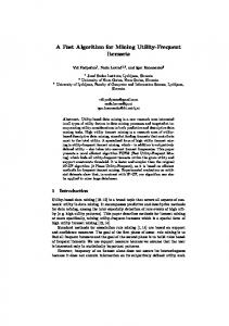
Execution times on T15N150D100K

As shown in Fig. 2, on T15N150D100K, for minimum utility thresholds between 2% and 6%, IHUI-Mine is 2.74, 2.90, and 2.19 times faster than Two-Phase, HUC-Prune, and UMMI, respectively. In this set of experiments, FUM is faster than Two-Phase, HUC-Prune, and UMMI and is 31% slower than IHUI-Mine. This is because the IIDS strategy used by FUM is more suitable for this sparse dataset than the pattern-growth method used by HUC-Prune and maximal itemset method used by UMMI.

T10N100D1M Two-Phase FUM HUC-Prune UMMI IHUI-Mine

2500

Execution time(sec)

2000

1500

1000

500

0 38

36

34

32

30

28

26

24

22

20


Fig. 3

Execution times on T10N100D1M

17

18

16

As shown in Fig. 3, on T10N100D1M the execution times of Two-Phase and FUM still significantly increase with decreasing minimum utility threshold, and both of these algorithms are an order of magnitude slower than IHUI-Mine when the minimum threshold is lower than 20%. While the remaining algorithms demonstrate relatively steady execution times, IHUI-Mine is still more efficient than HUC-Prune and UMMI. The reason is that the subsume index structure used in IHUI-Mine is less sensitive to the increase in total HUIs seen in T10N100D1M.

T15N150D100K

1200

Two-Phase FUM HUC-Prune UMMI IHUI-Mine

1100 1000

Memory usage(MB)

900 800 700 600 500 400 300 200 100 0 6.5

6.0

5.5

5.0

4.5

4.0

3.5

3.0

2.5

2.0

1.5

18

16


Memory usage on T15N150D100K

Fig. 4

T10N100D1M

900


800

Memory usage(MB)

700 600 500 400 300 200 100 38

36

34

32

30

28

26

24

22

20


Fig. 5

Memory usage on T10N100D1M

18

We also compared the memory usage of the five algorithms on the synthetic datasets (Figs. 4 and 5). These figures show that IHUI-Mine uses less memory than the other four algorithms. The main reason is that the additional memory required for the subsume index is less than that for either the original database or tree structures. Furthermore, by exploiting the subsume index the IHUI-Mine algorithm can find HUIs with only a small additional load, and it can also effectively eliminate many unpromising candidate itemsets through enumeration and pruning strategies. The tree-based HUC-Prune algorithm consumes more memory than any of the other four algorithms on T15N150D100K. This result is caused by the poor compression effect of HUC-Trees on this sparse synthetic dataset. From the above discussion, it can been seen that IHUI-Mine outperforms Two-Phase, FUM, HUC-Prune, and UMMI with regard to both efficiency and memory usage on synthetic datasets. 5.3 Performance analysis on real datasets

We next compare performance on dense real-world datasets: Mushroom, BMS-POS, and Chain-store. As the probability of an item’s occurrence in each transaction in these datasets is high, the run times tend to be long, especially when the minimum utility threshold is low. Furthermore, these real datasets also generate a large number of candidates. Figs. 6–8 show the execution time comparisons, with IHUI-Mine achieving the best performance.

Mushroom

4000


3500

Execution time(sec)

3000 2500 2000 1500 1000 500 0 30

28

26

24

22

20

18

16

14


Fig. 6

Execution times on Mushroom

19

12

10

As shown in Fig. 6, IHUI-Mine is an order of magnitude faster than Two-Phase, FUM, and UMMI on average for the Mushroom dataset. IHUI-Mine is 4.83 times faster than HUC-Prune on average; when the minimum utility threshold is 10%, IHUI-Mine is also an order of magnitude faster than HUC-Prune. This is because there are more co-occurring items in Mushroom than in other datasets, which enables the significant efficiency improvement offered by use of the subsume index.

BMS-POS

1800


1600

Execution time(sec)

1400 1200 1000 800 600 400 200 26

24

22

20

18

16

14

12

10

8


Fig. 7

Execution times on BMS-POS

As shown in Fig. 7 for BMS-POS, IHUI-Mine runs almost six times faster than Two-Phase, five times faster than FUM, four times faster than UMMI, and twice as fast as HUC-Prune. Although the execution times of both IHUI-Mine and HUC-Prune are nearly constant, IHUIMine is always faster than HUC-Prune.

20

Chain-store 9000

HUC-Prune UMMI IHUI-Mine

8000

Execution time (sec)

7000 6000 5000 4000 3000 2000 47.0

46.8

46.6

46.4

46.2

46.0

45.8

45.6

45.4

45.2

Minimum utility threshold (%)

Fig. 8

Execution times on Chain-store

Figure 8 shows the execution times for the Chain-store dataset. In this set of experiments we only report the results of IHUI-Mine, HUC-Prune, and UMMI: Two-Phase always takes an enormous amount of time (for example, for a minimum utility threshold of 47%, its execution time is over 5 h). FUM runs out of memory in several cases. Thus, these two algorithms are not included in this comparison. IHUI-Mine is faster than both HUC-Prune and UMMI for all utility thresholds. On average, IHUI-Mine is 1.31 times faster than HUC-Prune, and 2.58 times faster than UMMI. We also compared the memory usage for the three datasets (Figs. 9–11). As shown in Fig. 9, the amount of memory used on the Mushroom dataset by Two-Phase and FUM is nearly constant at over 200 MB. As the minimum utility threshold decreases, the memory consumption of UMMI ranges between 130 and 160 MB. Both HUC-Prune and IHUI-Mine use less memory than these three when the utility threshold is high. However, once the utility threshold decreases to 13%, the memory usage of HUC-Prune drastically exceeds that of IHUI-Mine.

21

Mushroom

300


270 240

Memory usage(MB)

210 180 150 120 90 60 30 0 30

28

26

24

22

20

18

16

14

12

10


Fig. 9

Memory usage on Mushroom

BMS-POS

450


400

Memory usage(MB)

350 300 250 200 150 100 50 0 26

24

22

20

18

16

14

12

10

8


Fig. 10 Memory usage on BMS-POS

On BMS-POS (Fig. 10), IHUI-Mine consumes, on average, one-quarter the memory of Two-Phase, one-third that of FUM, and one-fifth of that used by UMMI. IHUI-Mine uses slightly less memory than HUC-Prune, with the difference becoming more significant when the utility threshold is lower than 12%.

22

Chain-store 800

HUC-Prune UMMI IHUI-Mine

750 700

Memory usage (MB)

650 600 550 500 450 400 350 300 250 47.0

46.8

46.6

46.4

46.2

46.0

45.8

45.6

45.4

45.2

Minimum utility threshold (%)

Fig. 11 Memory usage on Chain-store

Figure 11 shows the memory usage for Chain-store as the minimum utility threshold decreases. As with the execution time results, we only plot the results for three algorithms (HUC-Prune, UMMI, and IHUI-Mine). IHUI-Mine uses around 59.01% of the memory used by HUC-Prune, and 44.50% of that used by UMMI. 5.4 Performance for different sorting methods

In the proposed IHUI-Mine algorithm, we sort items in order of ascending TWU during the entire mining process. To demonstrate the benefit of this strategy, we compare the performance of IHUI-Mine with different sorting strategies: lexicographic order (“IHUI-Mine-L”), descending TWU order (“IHUI-Mine-D”), and ascending TWU order (“IHUI-Mine”). Note that IHUI-Mine is used to denote the ascending-order implementation because this is the sorting strategy we selected for the final implementation. We conducted experiments on one synthetic dataset, T10N100D1M, and one real dataset, BMS-POS, because T10N100D1M is larger than its synthetic counterpart T15N150D100K, and BMS-POS is also larger than Mushroom.

23

T10N100D1M

1000 IHUI-Mine-L IHUI-Mine-D IHUI-Mine

900 800 Execution time(sec)

700 600 500 400 300 200 100 36

34

32

30

28

26

24

22

20

18


Fig. 12 Execution times of IHUI-Mine for different sorting methods on T10N100D1M

T10N100D1M


500 450 Memory usage(MB)

400 350 300 250 200 150 100 50 36

34

32

30

28

26

24

22

20

18


Fig. 13 Memory usage of IHUI-Mine for different sorting methods on T10N100D1M

As can be seen from Figs. 12 and 13, on the T10N100D1M dataset the TWU ascendingorder implementation is always faster and consumes less memory than the other two implementations. In Figs. 14 and 15, although the difference between IHUI-Mine-L and IHUIMine-D is not as significant as on T10N100D1M, both run time and memory consumption are best with the TWU ascending implementation on BMS-POS. Based on these data, we conclude

24

that ascending TWU order is superior to the other two implementations (lexicographic and descending TWU order).

BMS-POS


600

Execution time(sec)

500 400 300 200 100 0 26

24

22

20

18

16

14

12

10

8


Fig. 14 Execution times of IHUI-Mine for different sorting methods on BMS-POS

BMS-POS


160

Memory usage(MB)

140 120 100 80 60 40 20 26

24

22

20

18

16

14

12

10

8


Fig. 15 Memory usage of IHUI-Mine for different sorting methods on BMS-POS

25

5.5 Scalability

Finally, we discuss the results of tests conducted to verify the algorithms’ scalability. The datasets used for these tests were all generated by the IBM data generator (Agrawal and Srikant 1994). We varied the size of the T10N10 dataset to evaluate the scalability of the five algorithms discussed above. In this set of experiments, the number of transactions in T10N10 was increased from 50K to 2,000K, and the minimum utility threshold is set to 3%. Figures 16 and 17 show the execution times and memory requirements of the five algorithms as the number of transactions increases. As shown in Fig. 16, on average, IHUI-Mine is 5.50, 5.76, 1.37, and 2.73 times faster than Two-Phase, FUM, HUC-Prune, and UMMI, respectively. Meanwhile, as shown in Fig. 17, the memory requirements of IHUI-Mine are substantially lower than those of its competitors. These two plots strongly suggest that both the execution times and memory requirements of IHUI-Mine grow linearly with the size of the dataset.

T10N10D50K-2000K 2000


1800 1600

Execution time(sec)

1400 1200 1000 800 600 400 200 0 0

200

400

600

800

1000 1200 1400 1600 1800 2000

Number of transaction(K) Minimum utility threshold = 3%

Fig. 16 Execution time scalability for T10N10

26

T10N10D50K-2000K Two-Phase FUM HUC-Prune UMMI IHUI-Mine

1400

Memory usage(MB)

1200

1000

800

600

400

200

0 0

200

400

600

800

1000 1200 1400 1600 1800 2000

Number of transaction(K) Minimum utility threshold = 3%

Fig. 17 Memory usage scalability for T10N10

We also generated another data series, T15D100K, with a minimum utility threshold of 5%, to evaluate scalability. In these experiments, the number of items varied from 100 to 500. Figures 18 and 19 show the execution time and memory usage results for the five algorithms on T15D100K as the number of items increases. Interestingly, the execution time and memory usage of most of the algorithms decrease as the number of items increases. This is because the HUI distribution becomes sparser as the number of items increases. IHUI-Mine is more efficient and uses less memory than the other four algorithms throughout the range.

27

T15D100KN100-500 500


450 400

Execution time(sec)

350 300 250 200 150 100 50 0 100

200

300

400

500

Number of items Minimum utility threshold = 5%

Fig. 18 Execution time scalability for T15D100K

T15D100KN100-500 500


450 400

Memory usage(MB)

350 300 250 200 150 100 50 0 0

100

200

300

400

500

Number of items Minimum utility threshold = 5%

Fig. 19 Memory usage scalability for T15D100K

5.6 Summary of experimental results

The experimental results above demonstrate that IHUI-Mine outperforms existing state-ofthe-art algorithms in most cases on both synthetic and real datasets. The reasons can be summarized as follows. First, bitmap representations are used to compress the transaction database. Thus, storage requirements are reduced and efficient bitwise operations can also be exploited. Second, by using 28

the subsume index, co-occurring items can be identified efficiently. Theorem 2 can be subsequently used to enumerate HTWUIs directly by combination from the subsume index. As with the performance of frequent itemset mining algorithms (Song et al. 2008; Vo et al. 2013) based on this structure, the subsume index is particularly efficient when there are many cooccurring items. For example, on the Mushroom dataset, IHUI-Mine is an order of magnitude faster than the other four algorithms when the minimum utility threshold is 10%. Finally, Theorem 3 can be used to avoid unnecessary recursion, and Theorem 4 can be used to reduce the additional cost of storing intermediate results. We also analyzed the difference between IHUI-Mine and the tree-based algorithm HUCPrune (Ahmed et al. 2011). HUC-Prune is an efficient HUI mining algorithm based on FPGrowth (Han et. al 2004). It uses the HUC-Tree structure—a prefix tree storing the candidate items in descending TWU order. Every node in the HUC-Tree consists of an item name and a TWU value. The mining performance of HUC-Prune is closely related to the number of conditional trees constructed during the entire mining process and the construction/traversal cost of each conditional tree. When HUC-Tree compresses the original database successfully, the performance of HUC-Prune is good. In contrast, when the minimum utility threshold is very low, HUC-Tree becomes bushy. That is, there are few items sharing branches of the HUC-Tree. The overhead of the links increases the size of the HUC-Tree, degrading the performance of HUCPrune. As an example, the compression effect of HUC-Tree on T15N150D100K from the original database is not significant, leading to poor performance. In IHUI-Mine, the subsume index is only used for 1-HTWUIs and not recursively built for longer itemsets. Thus, the cost of generating the index is proportional to the number of 1HTWUIs. As reported in a recent study of frequent itemsets (Vo et al. 2013), the cost of generating the subsume index is relatively low even for sparse datasets with few elements in the subsume index. Moreover, for datasets with many co-occurring items (e.g., Mushroom), the effect of directly enumerating HTWUIs from the subsume index is significant. Furthermore, lowering the minimum utility threshold for a given dataset may increase the number of cooccurring items. In such cases, the advantages of IHUI-Mine are even more evident. The experimental results (Figs. 6 and 8) show that IHUI-Mine increasingly outperforms HUC-Prune as the minimum utility threshold decreases, supporting the above discussion. 29

6 Conclusions We have proposed an algorithm for mining high utility itemsets, IHUI-Mine. This algorithm uses the subsume index structure to identify items that co-occur with 1-HTWUIs. It also uses bitmap representations to calculate the subsume index. It is demonstrated that the subsume index can also be used to efficiently enumerate HTWUIs and avoid unnecessary recursion. As a result of these strategies and optimizations, IHUI-Mine outperforms other state-of-the-art algorithms and requires less memory. Finally, we also show that IHUI-Mine is scalable. Acknowledgments This work was partly supported by the National Natural Science Foundation of China (grant 61105045) and North China University of Technology (grant CCXZ201303).

Appendix A: Proof of Theorem 2 For Xsubsume(i), we have the following two cases. (1) The case that X=. Thus, iX= i, so we have TWU(i)=TWU(iX). (2) The case that X. Suppose X= b1b2…bk, where bjI(1jk). Since Xsubsume(i) for bjX, we have bjsubsume(i). According to Definition 2, g(i)g(bj). Thus, g(iX)=g(i)g(X)=g(i)g(b1)g(b2)…g(bk)=g(i) and we have TWU(i)=TWU(iX).

Appendix B: Proof of Theorem 3 We prove the theorem by contradiction. Suppose there exists jsubsume(i), such that ij is an HTWUI. Since the size of the set returned by the function g(X) (described in Section 4.1) decreases as the size of the itemset X increases, and iij, we have g(ij)



g(i), i.e.,

TWU(ij)TWU(i). Assume TWU(ij)=TWU(i), this means g(i)=g(ij)=g(i)g(j), which leads to g(i)g(j). According to Definition 2, we can easily find that jsubsume(i), which contradicts the hypothesis. Thus, TWU(ij)