Highly efficient and accurate spectral approximation of ... - Purdue Math

JOURNAL OF MATHEMATICAL STUDY J. Math. Study, Vol. x, No. x (201x), pp. 1-19

Highly efficient and accurate spectral approximation of the angular Mathieu equation for any parameter values q Haydar Alıcı1 and Jie Shen2 1

Department of Mathematics, Harran University, 63290 S¸anlıurfa, Turkey corresponding author. Department of Mathematics, Purdue University, 47907 West Lafayette, IN, USA 2

Abstract. The eigenpairs of the angular Mathieu equation under the periodicity condition are accurately approximated by the Jacobi polynomials in a spectral-Galerkin scheme for small and moderate values of the parameter q. On the other hand, the periodic Mathieu functions are related with the spheroidal functions of order ±1/2. It is well-known that for very large values of the bandwidth parameter, spheroidal functions can be accurately approximated by the Hermite or Laguerre functions scaled by the square root of the bandwidth parameter. This led us to employ the Laguerre polynomials in a pseudospectral manner to approximate the periodic Mathieu functions and the corresponding characteristic values for very large values of q. Key Words: Mathieu function; spectral methods; Jacobi polynomials; Laguerre polynomials AMS Subject Classifications: 33E10; 33D50; 65L60; 65L15

1

Introduction

Mathieu functions were first introduced by Mathieu in 1868 while investigating the vibrating modes of an elliptic membrane [32]. The eigenpairs of the Mathieu equation are needed in many scientific phenomena including wave motion in elliptic coordinates such as acoustic and electromagnetic scattering from an elliptic structures [14, 19, 26, 31], particle in a periodic potential [22] and vibrational spectroscopy of molecules with near resonant frequencies [37, 43]. Theoretical aspects of the Mathieu functions have been studied by many authors, including Stratton [42], McLachlan [33], Sips [41], Meixner & Sch¨afke [34] and Wang and Zhang [45] (cf. also [44]). As is seen for many physical and mathematical problems in elliptic geometries the separation of variables process in elliptic coordinates leads to the Mathieu equations. If one wants to solve these problems with large wavenumbers, it is very important to be able to obtain accurate numerical solutions for the angular Mathieu equation for very http://www.global-sci.org/ata/

1

c

201x Global-Science Press

2

H. Alıcı and Jie Shen / J. Math. Study, x (201x), pp. 1-19

large values of q since it is related to the wavenumber parameter present in these equations. Mathieu functions remain difficult to employ, mainly because of the impossibility of analytically representing them in a simple and handy way [41]. There are numerous studies on the numerical computation of the Mathieu functions and corresponding eigenvalues. Erricolo used Blanch’s algorithm for computing the expansion coefficients of Mathieu functions [16]. Erricolo and Carluccio provided software to compute angular and radial Mathieu functions for complex q values [17]. Shirts presented two algorithms for the computation of eigenvalues and solutions of Mathieu’s differential equation for noninteger orders [39, 40]. Alhargan introduced algorithms for the computation of all Mathieu functions of integer order which can deal with a range of the order n (0 − 200) and the parameter q (0 − 4n2 ) [3]. Co¨ısson and co-workers describe a numerical algorithm which allows a flexible approach to the computation of all the Mathieu functions [12]. Cojocaru in [13] provided Mathieu functions computational toolbox implemented in Matlab. MATSLISE is another software package for the computation of the Mathieu eigenpairs by using the power of high-order piecewise constant perturbation methods [29] and many others [1, 9, 21, 24, 25, 28, 30]. Most of the above algorithms employ the well-known trigonometric series representation

∞

ce2n (η,q) = ∑ A2k (q) cos(2kη ), k =0 ∞

(2n)

∞

ce2n+1 (η,q) = ∑ A2k+1 (q) cos[(2k + 1)η ] k =0 ∞

(2n+1)

se2n+1 (η,q) = ∑ B2k+1 (q) sin[(2k + 1)η ], se2n+2 (η,q) = ∑ B2k+2 (q) sin[(2k + 2)η ] k =0

(2n+1)

(2n+2)

k =0

(1.1) for computing the periodic Mathieu functions where A and B are known as the expansion coefficients. There are several ways of computing these expansion coefficients such as continued fractions method [33], the forward and the backward recurrence relations [9, 17] and as the eigenvectors of tri-diagonal matrix-eigenvalue problems [12, 13]. Each has its advantages and disadvantages. However, these algorithms are not suitable for very large values of q. Thus, the aim of this study is to construct accurate and efficient spectral algorithms for the computation of the integer order periodic Mathieu functions and the corresponding characteristic values for both small and very large values of the real parameter. The rest of the paper is organized as follows: Sections 2 and 3 are concerned with the construction of the spectral methods for small and very large values of q, respectively. Some numerical results are presented in Section 4. The last section concludes the paper with some remarks.

H. Alıcı and Jie Shen / J. Math. Study, x (201x), pp. 1-19

2

3

Spectral formulation for small and moderate parameter values

For any given value of the parameter q, the angular Mathieu equation d2 Φ +(λ − 2qcos2η )Φ = 0 dη 2

(2.1)

supplemented with a certain periodic boundary conditions admits two linearly independent families of periodic solutions with period π or 2π for specific values of the separation constant λ. Such values of the parameter λ are known as characteristic values or eigenvalues. When the solutions Φ(η ) are even with respect to η = 0 the characteristic values are denoted as an (q) whereas for odd solutions they are represented as bn+1 (q), n = 0,1,.... Periodic eigenfunctions corresponding to the an (q) and bn+1 (q) are denoted by cen (η;q) and sen+1 (η;q), respectively. The notations ce and se are due to Whittaker and Watson [47] and they stand for cosine-elliptic and sine-elliptic, respectively. Table 1: The periodic Mathieu functions. Boundary condition Φ0 (0;q) = Φ0 (π/2;q) = 0 Φ0 (0;q) = Φ(π/2;q) = 0 Φ(0;q) = Φ0 (π/2;q) = 0 Φ(0;q) = Φ(π/2;q) = 0

Mathieu functions ce2n (η;q) ce2n+1 (η;q) se2n+1 (η;q) se2n+2 (η;q)

Eigenvalues a2n (q) a2n+1 (q) b2n+1 (q) b2n+2 (q)

Character even ß − periodic even 2ß − periodic odd 2ß − periodic odd ß − periodic

Before describing the numerical scheme, we first transform the angular Mathieu equation to a more tractable form for each boundary condition set in Table 1. The angular Mathieu equation in (2.1) and Table 1 allow us to write 00 +( a2n − 2qcos2η )ce2n = 0, ce2n

0 0 ce2n (0;q) = ce2n (π/2;q) = 0.

(2.2)

that can be transformed to an equivalent algebraic form 1 (1 − x2 )y00n − xy0n − qxyn = µn (q)yn , 2

1 µn (q) = − a2n (q) 4

(2.3)

by the mapping x = cos2η ∈ (−1,1) where yn ( x;q) = ce2n ( x;q). The connection formula ce2n (η;q) = Cyn (cos2η;q)

(2.4)

reveals that the function u does not have to satisfy any boundary conditions at all. Next, we consider the system 00 ce2n +1 +( a2n+1 − 2qcos2η ) ce2n+1 = 0,

0 ce2n +1 (0;q ) = ce2n+1 ( π/2;q ) = 0

(2.5)

and have found the corresponding algebraic form to be 1 (1 − x2 )y00n +(1 − 2x )y0n − qxyn = µn (q)yn , 2

1 µn (q) = [1 − a2n+1 (q)] 4

(2.6)

4

H. Alıcı and Jie Shen / J. Math. Study, x (201x), pp. 1-19

upon use of the transformations x = cos2η and ce2n+1 ( x;q) = (1 + x )1/2 yn ( x;q) on both independent and dependent variables, respectively. Returning back to the original variables we see that the solution √ ce2n+1 (η;q) = C ( 2cosη )yn (cos2η;q) (2.7) satisfies the boundary conditions in (2.5) meaning that we don’t need to impose any boundary conditions on (2.6). Thirdly, the maps x =cos2η and se2n+1 ( x;q)=(1− x )1/2 yn ( x;q) transform the system 00 se2n +1 +( b2n+1 − 2qcos2η ) se2n+1 = 0,

0 se2n+1 (0;q) = se2n +1 ( π/2;q ) = 0

(2.8)

to the equivalent algebraic form 1 (1 − x2 )y00n −(1 + 2x )y0n − qxyn = µn (q)yn , 2

1 µn (q) = [1 − b2n+1 (q)] 4

without any boundary conditions since the solution √ se2n+1 (η;q) = C ( 2sinη )yn (cos2η;q)

(2.9)

(2.10)

readily satisfies the conditions in (2.8). Finally, the system 00 se2n +2 +( b2n+2 − 2qcos2η ) se2n+2 = 0,

se2n+2 (0;q) = se2n+2 (π/2;q) = 0

(2.11)

can be converted to the form 1 (1 − x2 )y00n − 3xy0n − qxyn = µn (q)yn , 2

1 µn (q) = [4 − b2n+1 (q)] 4

(2.12)

by means of x = cos2η and se2n+2 ( x;q)=(1 − x2 )1/2 yn (η;q). Again, the solution in original variable √ √ se2n+2 (η;q) = C ( 2sinη )( 2cosη )yn (cos2η;q) (2.13) satisfies the specified boundary conditions. Actually the equations in (2.3), (2.6), (2.9) and (2.12) can be put together to give the equation   2 d 1 (α,β) (α,β) (α,β) 2 d Lyn := (1 − x ) 2 +[ β − α −(α + β + 2) x ] − qx yn ( x;q) = µ(α,β) (q)yn ( x;q) dx dx 2 (2.14) with 1 µ(α,β) (q) = [(α + β + 1)2 − λ(q)]. (2.15) 4 The characteristic values λ(q) = { a2n (q),a2n+1 (q),b2n+1 (q),b2n+2 (q)}

(2.16)

H. Alıcı and Jie Shen / J. Math. Study, x (201x), pp. 1-19

5

of (2.1) are connected with those of the equation in (2.14) by the relations   (− 21 ,− 12 ) (− 21 , 12 ) ( 12 ,− 12 ) ( 21 , 21 ) −4µn (q),1 − 4µn (q),1 − 4µn (q),4 − 4µn (q)

(2.17)

respectively while the corresponding eigenfunctions Φ(α,β) (η;q) = {ce2n (η;q),ce2n+1 (η;q),se2n+1 (η;q),se2n+2 (η;q)}

(2.18)

are related with the solutions of (2.14) by the formula √ 1 √ 1 ( α,β ) Φ(α,β) (η;q) = C ( 2sinη )α+ 2 ( 2cosη ) β+ 2 yn (cos2η;q). (2.19)  1 1 Notice that, the set of parameter values (α,β) = (− 2 , − 2 ), (− 21 , 12 ), ( 12 , − 12 ), ( 12 , 21 ) lead to the eigenpairs (ce2n ,a2n ), (ce2n+1 ,a2n+1 ), (se2n+1 ,b2n+1 ) and (se2n+2 ,b2n+2 ), respectively. Here, the constant C will be chosen in such a way that ||Φ(η;q)|| L2 (0,π ) = π. That is, π=

Z 2π h 0

Φ

(α,β)

i2

(η;q) dη = 4

π 2

Z

h

0

= 4C2 = 2C2

i2 Φ(α,β) (η;q) dη π 2

Z

1

1

(2sin2 η )α+ 2 (2cos2 η ) β+ 2 y2n (cos2η )dη

0

Z 1 −1

y2n ( x )ω (α,β) ( x )dx = 2C2 ||yn ||2L2

ω (α,β)

(2.20)

(−1,1)

leading to r C=

π 2

(2.21)

when the orthonormal eigenfunctions ||yn || L2ω (−1,1) = 1 of (2.14) is in consideration. Now, we will construct the Galerkin spectral formulation of (2.14). Let (α,β) φk ( x ) =

1 (α,β) P ( x ), hk k

(α,β) hk =



2α + β +1 Γ ( k + α + 1) Γ ( k + β + 1) 2k + α + β + 1 k!Γ(k + α + β + 1)

 12

be the normalized Jacobi polynomials of degree k and order (α,β) and n o (α,β) X N = span φk ( x ) | k = 0,1,..., N .

(2.22)

(2.23)

(α,β)

The Spectral-Galerkin method for (2.14) is to find yn,N ∈ X N such that (α,β)

(α,β)

( Lyn,N , p N )ω(α,β) = µn

(α,β)

(yn,N , p N )ω(α,β) ,

∀ pN ∈ XN

(2.24)

where ω (α,β) ( x ) = (1 − x )α (1 + x ) β is the Jacobi weight function. Now, proposing (α,β)

yn

N

( x;q) ≈ yn,N ( x;q) = ∑ cnk φk (α,β)

k =0

(α,β)

( x ),

(2.25)

6

H. Alıcı and Jie Shen / J. Math. Study, x (201x), pp. 1-19

(α,β)

letting p N ( x ) = φj ( x ) and keeping in mind that the normalized Jacobi polynomials satisfy the differential equation 

(1 − x 2 )

 d d2 (α,β) φk ( x ) = 0 +[ β − α −( α + β + 2 ) x ] + k ( k + α + β + 1 ) dx2 dx

(2.26)

we see that the Spectral-Galerkin formulation (2.24) of the differential eigenvalue problem (2.14) reduces to the matrix-eigenvalue equation

(S + R)cn = µn cn

(2.27)

with cn = (cn0 ,cn1 ,...,cnN )T , S = [S jk ] = −k (k + α + β + 1)δjk and 1 R = [ R jk ] = − q 2

Z 1 −1

(α,β)

xφk

(α,β)

( x )φj

( x )ω (α,β) ( x )dx.

(2.28)

The three term recurrence relation of the normalized Jacobi polynomials (α,β) (α,β) (α,β) (α,β) (α,β) (α,β) φk+1 ( x )+( Bk − x )φk ( x )+ Ak−1 φk−1 = 0,

Ak

(α,β)

φ0

=

1 (α,β) h0

,

(α,β)

φ1

(x) =

1 (α,β) 2h1

[(α + β + 2) x + α − β]

(2.29)

in which   21 2 β2 − α2 k (k + α)(k + β)(k + α + β) (α,β) = ,Bk 2k + α + β (2k + α + β − 1)(2k + α + β + 1) (2k + α + β)(2k + α + β + 2) (2.30) allows us to write down the entries  (α,β) 1  Ak , j = k + 1 R jk = Rkj = − q (2.31) 2  (α,β) Bk , j = k (α,β) A k −1 =

of the symmetric tri-diagonal matrix R for j,k =0,1,..., N. Notice in (2.31) that the diagonal (α,β) entries are all zero since we have Bk = 0 for all k when (α,β) = (± 21 , ± 12 ) . Moreover, the entries of the matrix R requires special attention when (α,β) = (− 21 , − 12 ), since in this (−1/2,−1/2) √ (−1/2,−1/2) case the first coefficient A0 = 2/2 while Ak = 1/2 for k ≥ 1. The matrices have simple structure, more specifically S is a diagonal and R is a tridiagonal matrix with zero main diagonal. Thus, the resulting discrete system is a tridiagonal matrix. Despite its simple structure, the present formulation yields highly accurate numerical eigenpairs. For small q values, even the last discrete eigenpair corresponding to N is correct up to some digits which is promising if we remember the fact that only the two-thirds, often one-half or considerably smaller portion of the computed

H. Alıcı and Jie Shen / J. Math. Study, x (201x), pp. 1-19

7

Table 2: The number of eigenvalues (ev) having relative errors of order 10−14 and the number of eigenvectors (ef) having absolute errors of order at most 10−13 for a given truncation order N and the parameter q. N 100 300 600

q=1 ev ef 99 95 299 295 599 595

q = 102 ev ef 94 90 292 288 596 592

q = 103 ev ef 85 84 290 285 594 588

q = 104 ev ef 35 30 279 274 585 578

q = 105 ev ef 6 2 134 127 535 523

q = 106 ev ef 1 1 25 22 140 133

eigenpairs are correct up to some accuracy for a fixed truncation order N [10, 46]. Specifically, when q = 1 and N = 100, relative errors for all the eigenvalues except the last one are of order 10−14 and for the same N with q = 102 , ninety-four of them have relative errors of order 10−14 . On the other hand, the number of accurate aigenvectors having the values of the Mathieu functions at some evaluation points is slightly less than that of eigenvalues. The accuracy of the eigenpairs are checked by increasing the truncation order N systematically and observing the stable digits between two consecutive truncation orders N and N + 1. For the eigenvectors, vector infinity norm is used to measure the errors. Nevertheless, it can be seen from Table 2 that the number of accurate pairs decreases with a further increment in q. Indeed, a dramatic decrease occurs especially for q ≥ 105 . Therefore, in this article such q values will be called very large. Actually, the accuracy loss for large values of the parameters is typical for all parameter dependent problems such as the Coffey-Evans [18] and the prolate spheroidal wave equation. Efficient numerical approximation of the latter for very large values of the bandwidth parameter may be found in [4, 27, 35]. An efficient method for very large values of the parameter q will be derived in the next section.

3

Spectral formulation for very large parameter values

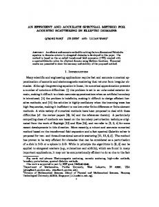
The main difficulty for very large q values originates from the fact that the eigenfunctions of (2.1) are confined to a small interval around the points η = π/2 and η = 3π/2 when they are considered in the interval (0,2π ) (see Fig. 1). Therefore, one has to focus on these portions of the interval. One remedy might be the use of mapped Jacobi pseudospectral methods by using a suitable mapping such as the one introduced in [7] which can clusters more points around a desired point. However, here we are in favor of employing another technique which is more efficient and accurate from the numerical point of view. Consider the general equation 

 d2 d ν2 2 2 − 2 + tanθ + + c sin θ Ψνn (θ;c) = λn (ν;c)Ψνn (θ;c) dθ dθ cos2 θ

(3.1)

8

H. Alıcı and Jie Shen / J. Math. Study, x (201x), pp. 1-19

(a) se1 (η,1)

(b) se1 (η,105 )

Figure 1: se1 (η,q) for specified values of q on [0,2π ]. where c and ν > −1 is a real parameter. The maps t = sinθ and Ψνn (θ;c) = (1 − t2 )ν ψνn (t;c) takes the equation to the algebraic form 00 0 (1 − t2 )ψνn − 2(ν + 1)tψνn − c2 t2 ψνn = µn (ν;c)ψνn

(3.2)

where µn (ν;c) = ν(ν + 1)− λn (ν;c). Stratton [42] and later Chu and Stratton [11] defined the spheroidal functions as the solutions of the last equation that remains finite at the singular points t = ±1. For integral orders ν = m = 0,1,2,... the functions ψνn (t;c) are related to the spheroidal wave functions that arise from separation of the Helmholtz equation in spheroidal coordinates. For half-integer values ν = ± 21 they are related to the angular Mathieu functions that arise from separation of the Helmholtz equation in elliptic coordinates [38]. Thus, we may make use of (3.1) to approximate the eigenpairs of the angular Mathieu equation for very large values of q whose details will be explained below. Note that, the solutions ψνn of (3.2) that remain finite at the end points t = ±1 suggest the use of boundary conditions Ψνn (±π/2;c) = 0 for (3.1). This makes equation (3.1) into a reflection symmetric system so that the even and odd states can be separated. Actually the transformations x = − cos2θ and Ψν2n ( x;c) = (1 − x )ν/2 yνn ( x ) lead to the equation

(1 − x

2

)y00νn +

        1 3 c2 1 c2 0 − ν+ − ν+ η yνn − xyνn = ν(ν + 1)+ − λ2n (ν;c) yνn (3.3) 2 2 8 4 2

where x ∈(−1,1). On returning back to the original variables Ψν2n (θ;c)=cosν θyνn (− cos2θ ), we see that the even indexed eigenfunctions are even functions of θ. For the odd states, first we use the map Ψν2n+1 (θ;c) = sinθφν2n+1 (θ;c) = where φν2n+1 is necessarily an even function of θ. This suggest use of the same transformations employed for the even states

H. Alıcı and Jie Shen / J. Math. Study, x (201x), pp. 1-19

9

leading to the equation         1 1 5 c2 c2 0 (1 − x − ν− − ν+ η yνn − xyνn = (ν + 1)(ν + 2)+ − λ2n+1 (ν;c) yνn 2 2 8 4 2 (3.4) where the odd state eigenfunctions Ψν2n+1 (θ;c) = sinθcosν θyνn (− cos2θ ) are indeed an odd function of θ. Therefore, instead of (3.2), we have two equations to handle the even and odd states of (3.1) separately. Actually the last two equations can be unified as 2



)y00νn +

 d2 d 1 2 (α,β) (α,β) (1 − x ) 2 +[ β − α −(α + β + 2) x ] − c x yn ( x;q) = µ(α,β) (ν;c)yn ( x;q) dx dx 8 2

in which µ(α,β) (ν;c) =

1 4

 α+ β+

1 2

 α+ β+

  3 − λ(ν;c) 2

(3.5)

(3.6)

where the parameters (α,β) = (ν, − 21 ) and (α,β) = (ν, 21 ) yield the even and odd states, respectively. Now, taking c2 = 4q and comparing (3.5)-(3.6) with (2.14)-(2.15) we obtain the connection relations     1 1 p 1 1 p a2n (q) = − 2q + λ2n − ; 4q , b2n+1 (q) = − 2q + λ2n ; 4q 4 2 4 2     (3.7) 1 1 1 p 1 p a2n+1 (q) = − 2q + λ2n+1 − ; 4q , b2n+2 (q) = − 2q + λ2n+1 ; 4q 4 2 4 2 among the eigenvalues of the Mathieu and the generalized spheroidal equation in (3.1). Meanwhile, the well-known relations [33] a2n (−q) = a2n (q),

a2n+1 (−q) = b2n+1 (q),

b2n+2 (−q) = b2n+2 (q)

(3.8)

among the eigenvalues of the Mathieu equation, together with (3.7) lead to the interesting relations         1 1 1 1 λ2n − ;c − λ2n − ;ic = c2 , λ2n+1 − ;c − λ2n ;ic = c2 2 2 2 2         (3.9) 1 1 1 1 2 2 λ2n ;c − λ2n+1 − ;ic = c , λ2n+1 ;c − λ2n+1 ;ic = c 2 2 2 2 among the eigenvalues of (3.1) when ν = ±1/2. For the spheroidal wave equation, that is when ν = m = 0,1,2,... in equation (3.1), we have presented highly accurate and efficient method for very large values of the bandwidth parameter c [4]. It was based on the idea that when c tends to infinity, the prolate spheroidal wave functions can accurately be approximated by the Hermite functions

10

H. Alıcı and Jie Shen / J. Math. Study, x (201x), pp. 1-19

scaled by the square root of the parameter c [6, 15, 20, 27, 36]. Clearly, they can also be approximated by the Laguerre functions of order ± 21 due to the connections (− 12 )

H2n ( x ) = (−1)n 22n n!Ln

( x 2 ),

(1)

H2n+1 ( x ) = (−1)n 22n+1 n!xLn2 ( x2 )

(3.10)

between the Hermite and Laguerre polynomials. The same idea can be used with ν = ± 12 to approximate the eigenpairs of the Mathieu equation as well. To this end, we transform the equation in (3.1) to another one over the positive half line. This can be accomplished by the maps x = [αarctanh(sinθ )]2 , x ∈ (0,∞) (3.11) and Ψνn ( x;c) = x a φνn ( x;c)

(3.12)

applying in respective order. The first map leads to the operational equivalence    2  d2 d 1 d d cos2 θ − 2 + tanθ ≡ −4α2 x 2 + dθ dθ dx 2 dx

(3.13)

for the differential part of (3.1) which is not the case for the operator d2 /dη 2 present in the angular Mathieu equation in (2.1). That is to say, in this case it is not possible to find a transformation from the interval η ∈ (0,π/2) to the half line x ∈ (0,∞) leading to such an operator with linear and constant polynomial coefficients. That is why we make use of the more general equation in (3.1) and finally take ν = ± 12 since in these two cases the solutions of (3.1) are related with the angular Mathieu functions. Application of the above transformations lead to the equation (γ)

00 0 xφνn +(γ + 1) φνn + Q( x )φνn = µn (ν;c)r ( x )φνn

where Q( x ) = −

(γ)

µn (ν;c) = −

1 λn (ν,c) 4α2



i 1 h 2 2 2 √ 2 √ ν + c sech x/α tanh x/α , 4α2 √
r ( x ) = sech2 x/α

(3.14)

(3.15) (3.16)

and γ = 2a − 12 . Clearly, γ = − 21 leads to the even-states whereas γ = 12 yield odd-states of (3.1) which can be seen on returning back to the original variables via (3.11)-(3.12). The eigenvalues of (3.1) are related with those of (3.14) by the formula (−1/2)

λ2n (ν,c) = −4α2 µn

(ν;c),

(1/2)

λ2n+1 (ν,c) = −4α2 µn

(ν;c)

(3.17)

from which we can compute the characteristic values p of the Mathieu equation employing 1 the connection formula (3.7) with ν = ± 2 and c = 4q. Here, α is a scaling or an optimization parameter whose optimum value is usually determined by trial and error. However, fortunately, for this problem as is explained

H. Alıcı and Jie Shen / J. Math. Study, x (201x), pp. 1-19

11

√ above its optimum value is fixed as αopt = c = (4q)1/4 . To approximate the eigenpairs of (3.14), we utilize the Laguerre functions in a pseudospectral picture since it reduces to the differential equation for the Laguerre functions when q( x ) ≡ 0 and r ( x ) = 1. Basically, the idea is to collect the grid points, that are the roots of the order γ = ±1/2 Laguerre polynomials, to the small interval where the eigenfunctions are away from zero by means √ of the scaling factor αopt = c. Now, consider the weighted interpolation of the solution of (3.14) N

N φνn ( x,c) = ∑ `k ( x )φνn ( xk ,c)

(3.18)

k =0

in which

`k ( x ) =

(γ) Lˆ N +1 ( x ) (γ) ( x − xk )∂ x Lˆ N +1 ( xk )

,

(γ) Lˆ N +1 ( x ) =

1 h N +1

(γ)

e− x/2 L N +1 ( x ),

h2N +1 =

Γ ( N + γ + 2) ( N + 1) !

(3.19) are the set of N −th degree Lagrange polynomials and xk stand for the N + 1 real and dis(γ) tinct roots of L N +1 ( x ) which are computed by using the well-known Golub-Welsch algorithm [5,23]. Proposing the interpolant as an approximate solution to (3.14) and requiring the satisfaction of (3.14) at the collocation points xk , we obtain a discrete representation (γ) Bˆ uˆ n = µn (ν;c)uˆ n

(3.20)

where uˆ n = [φνn ( x0 ,c) φνn ( x1 ,c) ... φνn ( x N ,c)] T contains the values of an eigenfunction at the nodal points. Then approximate eigenvalues λ2n (ν,c) and λ2n+1 (ν,c) of (3.14) may be determined from (3.20) with γ = − 21 and γ = 12 , respectively. After some algebra one may express the entries of the matrix B as  (γ)  −2xm ∂ x Lˆ N +1 ( xm )   if m 6= n   ( x m − x n )2 ˆ ( γ ) ∂ x L N +1 ( x n ) 2 √ ˆ Bmn = cosh ( xm /α) (3.21)   2    1 − γ − 2N + γ + 3 + xn + Q( xn ) if m = n 6xn 6 12 where Q( xn ) are the values of the function Q( x ) in (3.15) at the nodal points xn . This matrix can be factored as Bˆ = SB S−1 where S = diag{s1 ,s2 ,...,s N } is diagonal matrix with sm =

√

√ (γ) xm cosh ( xm /α) ∂ x Lˆ N +1 ( xm ),

m = 0,1..., N

and B is symmetric matrix with entries √ √ √  −2 xm xn cosh ( xm /α) cosh ( xn /α)   if m 6= n   ( x m − x n )2 Bmn =    1 − γ2 2N + γ + 3 xn  2 √   cosh ( xn /α) − + + Q( xn ) if m = n. 6xn 6 12

(3.22)

(3.23)

12

H. Alıcı and Jie Shen / J. Math. Study, x (201x), pp. 1-19

Therefore we may replace the unsymmetric system in (3.20) with the symmetric one (γ)

B un = µn (ν;c)un

(3.24)

since the similar matrices share the same eigenvalue set. Clearly, an eigenvector uˆ n of (3.20) is connected with that of (3.24) by uˆ n = Sun .

(3.25)

On the other hand, for an orthonormal eigenfunction of (3.14) we may write 1=

Z ∞ 0

2 φνn ( x;c) sech2

√




x/α x

2a− 21 − x

e

dx =

Z ∞ 0

Ψ2νn ( x;c) sech2

√


1 x/α x − 2 dx

(3.26)

√ where we have used (3.12). However, applying the change of variable sinθ = tanh( x/α) in (3.11), to an eigenfunction of (3.1) we obtain Z

π 2

Ψ2νn (θ;c) cosθdθ =2 π

π 2

Z

−2

1 = α

0

Ψ2νn (θ;c) cosθdθ

Z ∞ 0

Ψ2νn ( x;c) sech2

√




x/α x

− 12

1 dx = . α

(3.27)

√ This means that Ψνn (θ;c) = αΨνn ( x;c) so that the L2cosθ (−π/2,π/2) norm of the eigenfunction Ψνn (θ;c) in the original variable θ is unity. Thus, we may write √ √ 1 (γ+ 32 ) √ (γ) Ψνn (θm ;c) = αΨνn ( xm ;c) = αxm2 (3.28) cosh ( xm /α) ∂ x Lˆ N +1 ( xm )unm √ where θm = xm /α and unm is the m−th entry of the eigenvector un of (3.24). Actually an eigenvector of (3.24) depends on the parameters ν and γ, too. Hence, it is better to adopt (ν,γ) the notation un := un . Finally, using the differential-difference relation q (γ) (γ) (γ) (3.29) x∂ x Lˆ n ( x ) = n Lˆ n ( x )− n(n + γ) Lˆ n−1 ( x ) of the normalized Laguerre functions in (3.19) with n = N + 1 and x = xk , we may represent the angular Mathieu functions in terms of the spheroidal functions of orders ν = ±1/2 as √ p (ν,γ) Φn (θm ;q) = π/2Ψνn (θm ; 4q) q (3.30) 1 √ (γ− 21 ) (γ) (ν,γ) = − απ ( N + 1)( N + γ + 1)/2 xm2 cosh ( xm /α) Lˆ N ( xm )unm where the parameters (ν,γ) = {(− 21 , − 12 ), (− 21 , 12 ), ( 12 , − 21 ), (− 12 , 12 )} lead to the Mathieu functions Φ(ν,γ) = {ce2n ,ce2n+1 ,se2n+1 ,se2n+2 }, respectively, for very large values of the (γ) parameter q. Here, the values Lˆ N ( xm ) of the N −th normalized Laguerre function of order γ are computed in a stable way by using the recurrence q q (γ) (γ) (γ) (n + 1)(n + γ + 1) Lˆ n+1 ( x ) = (2n + γ + 1 − x ) Lˆ n ( x )− n(n + γ) Lˆ n−1 ( x ) (3.31)

H. Alıcı and Jie Shen / J. Math. Study, x (201x), pp. 1-19

13

where (γ) Lˆ 0 ( x ) = e− x/2 /

q

Γ ( γ + 1),

(γ) Lˆ 1 ( x ) = (γ + 1 − x )e− x/2 /

q

Γ ( γ + 2).

(3.32)

The matrix in (3.23) only necessitates the knowledge of the zeros of the ( N + 1)−st degree Laguerre polynomial of order γ = ±1/2. It is easy to construct and symmetric with quite reasonable condition number. In fact, numerical experiments reveal that as q gets larger, the condition number of the matrix B of size ( N + 1)×( N + 1) converges to 4N + 1 and (4N + 3)/3 when γ = −1/2 and γ = 1/2, respectively. Table 3: The number of eigenvalues having relative errors of order 10−14 for a given truncation order N and the parameter q. N 100 300 600

q = 105 Jacobi Laguerre 6 55 134 120 535 160

q = 106 Jacobi Laguerre 1 75 25 200 140 330

q = 1010 Jacobi Laguerre 90 265 585

Now, in Table 3 by comparing with the Jacobi spectral method we see that the Laguerre pseudospectral formulation leads to much better results for large q values, especially as q gets larger and larger.

4

Numerical results

In this section we present some numerical tables and plots of eigenfunctions for small, moderate and very large values of the parameter q. It is clear from Table 4 that the algorithms mentioned in this study can accurately approximate the eigenvalues when the parameter q is small. Here we executed our algorithm in Fortran quadruple precision arithmetic to see if the results agree with those of [1] up to the accuracy quoted. This does not mean that the other algorithms can not attain such accuracy for small q. In contrast, there would have been algorithms cited in this study which can also attain the same accuracy if they were implemented in quadruple precision arithmetic, too. Then in Table 5 we present the discrete values of the function ce9 (η,100) at the specified angles. First two columns include the results obtained from the present JacobiGalerkin method with the truncation orders N = 25 and N = 26. The last column includes the results from [8] which truncates the second series in (1.1) at N = 20. Although it seems that, our method yields better results then the classical trigonometric series expansion, at a cost of computing more expansion coefficients, the trigonometric series can also produce results that are accurate to machine precision. It is clear from Table 5 that for small values of q both the present Jacobi-Galerkin and the trigonometric series approach produce similar results.

14

H. Alıcı and Jie Shen / J. Math. Study, x (201x), pp. 1-19

Table 4: Comparison of b2 (25) and b10 (25) with some literature results. n b2n+2 (25) 0 -21.314860622249850854314664972573 -21.31486062224985085431466497257381226977 -21.31486062 -21.314860622 -21.3148606222499 -21.3148606222498 -21.31486062224972 4 103.225680042373470004799730544439 103.2256800423734700047997305444380455190 103.22568004 103.225680042 103.225680042418 103.225680042373 103.22568004237351

Reference Present Jacobi-Galerkin formulation [1] [2] [30] [24] [13] [29] Present Jacobi-Galerkin formulation [1] [2] [30] [24] [13] [29]

Table 5: Values of the Mathieu function ce9 (η,100) at the specified angles η. η 0◦ 10◦ 20◦ 30◦ 40◦ 50◦ 60◦ 70◦ 80◦

ce9 (η,100) N = 25 0.066266491141916 0.152283208659798 0.531438482965942 1.212916357317376 0.842535893157752 -0.955912622210367 0.439824653297739 -0.114071528013408 0.004366328988792

ce9 (η,100) N = 26 0.066266491141915 0.152283208659799 0.531438482965944 1.212916357317379 0.842535893157752 -0.955912622210367 0.439824653297739 -0.114071528013409 0.004366328988792

ce9 (η,100) Ref. [8] 0.066266491106052 0.152283208636151 0.531438482970954 1.212916357348340 0.842535893193692 -0.955912622195211 0.439824653279982 -0.114071528052211 0.004366328957511

Table 6 demonstrates the accuracy improvement of b2n+1 (q) for the parameter values q = 1,1010 and eigenvalue indices n = 1,1001. It is clear that the methods described here not only yield accurate results for lower states, but also for higher ones as high as thousand with quite reasonable truncation orders N. As a result of separation, the necessary truncation size to print b1001 (1) on the screen is N = 501. However, N = 502 is enough to obtain it with a relative error of order 10−15 . Similarly, N = 513 does the same job for b1001 (1010 ) revealing the efficiency of our algorithms. For comparison, the bottom row includes the results obtained from MATSLISE package [29] and Cojocaru [13]. The latter diagonalizes the tri-diagonal matrix resulted from writing the recurrence relation of the expansion coefficients of (1.1) in matrix form. As it is mentioned in Introduction, this type of approaches are suitable for small or moderate

H. Alıcı and Jie Shen / J. Math. Study, x (201x), pp. 1-19

15

Table 6: Accuracy improvement for b1001 (q) for q = 1 and q = 1010 by using the Jacobi and the Laguerre bases, respectively. N b1001 (1) 504 1002001.0000004984 505 1002001.0000004998 506 1002001.0000004988 1002001.0000004990a 505 1002001.00000050b

N 6 7 8 1100

b1 (1010 ) N -19999800000.250004 513 -19999800000.250008 514 -19999800000.250000 515 -19999800000.250000a -19999800000.249931b

b1001 (1010 ) -19600301128.153511 -19600301128.153587 -19600301128.153591 -19600301128.153572a − a

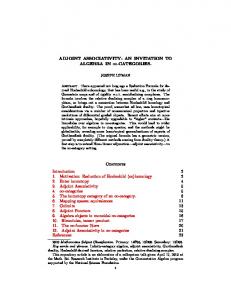
(a) ce30 (η,106 )

Reference [29], b Reference [13]

(b) ce50 (η,106 )

Figure 2: ce30 (η,106 ) and ce50 (η,106 ) corresponding to the characteristic values a30 (106 )= −1878467.04186782 and a50 (106 ) = −1799283.43142027, respectively. q values and not able to produce satisfactory results for very large values of the parameter q. Specifically, N = 2000 was not enough to approximate the eigenvalue b1001 (1010 ). Even for the ground state eigenvalue b1 (1010 ) one needs to diagonalize a matrix of size N = 1100. Actually, MATSLISE works for very large values of q as high as 1013 beyond which it also has difficulties in approximating the Mathieu eigenpairs. For large values of q it is still possible to approximate the lower eigenpairs by the Jacobi bases at a cost of very high truncation orders. In Fig. 2 we present plots of the Mathieu functions ce30 (η,106 ) and ce50 (η,106 ) that are obtained by using both the Jacobi and the Laguerre bases. Note the confinement of the eigenfunctions to a small interval around the point π/2 for such large values of q. In order to check the efficiency of the Laguerre basis approach, in Table 7 we include several eigenvalues for very large value of q = 1020 . In this case, the integer part of the eigenvalues occupy more than twenty digits. Therefore, we have implemented our algorithm in Fortran programming language by using quadruple precision arithmetic and tabulate the values a(q)+ 2q or b(q)+ 2q instead of a(q) and b(q), respectively. To ap-

16

H. Alıcı and Jie Shen / J. Math. Study, x (201x), pp. 1-19

Table 7: Several eigenvalues of the angular Mathieu equation for q = 1020 . N 5 55 255 505

n 0 100 500 1000

a2n (q)+ 2q ≈ b2n+1 (q)+ 2q 19999999999.7499999999968 4019999994949.7499936553094 20019999874749.7492164015471 40019999499499.7437406154262

a2n+1 (q)+ 2q ≈ b2n+2 (q)+ 2q 59999999998.749999999972 4059999994848.749993464034 20059999874248.749211695272 40059999498498.743721827900

proximate the eigenvalue a1000 (1020 ) with the present Laguerre pseudospectral method to the accuracy quoted, we only need to diagonalize a matrix of size 505 × 505 which is impressing. It is known that, for finite n and large q values a2n (q) ≈ b2n+1 (q) and a2n+1 (q) ≈ b2n+2 (q) [33]. This can also be observed from the equations (3.14)-(3.16) and (3.7). In fact, in (3.14) one has λn (ν,c) = λn (−ν,c) since there is a quadratic dependence on ν. Then, it is easy to see that an (q) ≈ bn+1 (q) by employing this fact in the connection formulas (3.7). Numerical results in Table 7 are in accordance with the asymptotic formula an (q) ≈ bn+1 (q) =− 2q + 2q1/2 k − 2−3 (k2 + 1)− 2−7 q−1/2 k (k2 + 3)

− 2−12 q−1 (5k4 + 34k2 + 405)− 2−17 q−3/2 k(33k4 + 410k2 + 405)+ O(q−2 ) (4.1) up to their last digits where k = 2n + 1 [28, 33]. Then, in Fig. 3 we present the plots of two eigenfunctions corresponding to the same q = 1020 . Notice in this case that their nonzero parts are confined to a tiny interval of length 10−4 around the points (2k + 1)π/2 where k is an integer.

(a) ce10 (η,1020 )

(b) se12 (η,1020 )

Figure 3: Mathieu functions ce10 (η,q) and se12 (η,q) corresponding to the characteristic values a10 (q)+ 2q = 419999999944.7499999927156 and b12 (q)+ 2q = 459999999933.7499999904406, respectively.

H. Alıcı and Jie Shen / J. Math. Study, x (201x), pp. 1-19

5

17

Conclusion

In this article, we have constructed accurate and efficient spectral and pseudospectral methods based on the Jacobi and the Laguerre polynomials to approximate the integer order periodic Mathieu functions and the corresponding characteristic values. To this end, the angular Mathieu equation is transformed into several equations resembling the Jacobi and the Laguerre differential equations. These particular transformations motivated us to use the most suitable Jacobi or Laguerre polynomial with specific parameter(s) as basis sets for the approximation of the eigenpairs. It is observed from numerical results that the Jacobi-Galerkin methods are well suited for small q values whereas the Laguerre pseudospectral methods scaled by (4q)1/4 are more appropriate for very large values of q. Note that, in the Laguerre pseudospectral method a suitable scaling parameter optimizing the accuracy is not chosen by experimentally since it is initially set as αopt = (4q)1/4 . The algorithms developed in this paper are implemented in a set of Matlab routines, Mathieu.m, Mathieu_Small_q.m, Mathieu_Large_q.m and eigfunplot.m, which can be downloaded via the link http://www.math.purdue.edu/~ shen/pub/mathieu.zip. The routine Mathieu.m serves as the main file which calls the other three to compute the Mathieu eigenpairs. Mathieu_Small_q.m and Mathieu_Large_q.m approximate the eigenpairs for |q| < 106 and |q| ≥ 106 , respectively whereas Eigfunplot.m is responsible for plotting the results obtained from these routines. The methods developed here will be useful in a variety of physical and engineering applications in which accurate solutions of the angular Mathieu equation are needed.

6

Acknowledgement

¨ ITAK, ˙ The first author’s research was supported by a grant from TUB the Scientific and Technological Research Council of Turkey. The second author’s research was partially supported by NSF DMS-1620262, DMS-1720442 and AFOSR FA9550-16-1-0102. References [1] A. A. Abramov and S. V. Kurochkin. Calculation of solutions to the mathieu equation and of related quantities. Comput. Math. and Math. Phys., 47(3):397–406, 2000. [2] M. Abramowitz and I. A. Stegun. Handbook of Mathematical Functions with Formulas, Graphs, and Mathematical Tables. Dover, New York, 1970. [3] F. A. Alhargan. Algorithms for the computation of all Mathieu functions of integer order. ACM Trans. Math. Softw., 26(3):390–407, 2001. [4] H. Alıcı and J. Shen. Highly accurate pseudospectral approximations of the prolate spheroidal wave equation for any bandwidth parameter and zonal wavenumber. J. Sci. Comput., 2016. doi:10.1007/s10915-016-0321-7. [5] H. Alıcı and H. Tas¸eli. The laguerre pseudospectral method for the radial schrodinger equation. Appl. Numer. Math., 87:87–99, 2015.

18

H. Alıcı and Jie Shen / J. Math. Study, x (201x), pp. 1-19

[6] B. E. Barrowes, K. O’Neill, T. M. Grzegorczyk, and J. A. Kong. On the asymptotic expansion of the spheroidal wave function and its eigenvalues for complex size parameter. Stud. Appl. Math., 113:271–301, 2004. [7] A. Bayliss and E. Turkel. Mappings and accuracy for Chebyshev pseudo-spectral approximations. J. Comput. Phys., 101(2):349–359, 1992. [8] M. M. Bibby and A. F. Peterson. Accurate Computation of Mathieu Functions. Morgan and Claypool, 2013. [9] G. Blanch. Numerical aspects of Mathieu eigenvalues. In Rend. Circ. Mat. Paler., 15:51–97, 1966. [10] J. P. Boyd. Computation of grid points, quadrature weights and derivatives for spectral element methods using prolate spheroidal wave functions-prolate elements. ACM Trans. Math. Softw., 31:149–165, 2005. [11] L. J. Chu and J. A. Stratton. Elliptic and spheroidal wave functions. J. Math. and Phys., 20:259–309, 1941. [12] R. Co¨ısson, G. Vernizzi, and X. Yang. Mathieu functions and numerical solutions of the Mathieu equation. Proc. IEEE Int. Workshop Open-Source Softw. Sci. Comput., pages 3–10, 2009. [13] E. Cojocaru. Mathieu functions computational toolbox implemented in Matlab. ArXiv:0811.1970, 2008. [14] R. Courant and D. Hilbert. Method of Mathematical Physics, volume Vol. 1. Wiley Interscience, 1966. [15] T. Do-Nhat. Asymptotic expansion of the Mathieu and prolate spheroidal eigenvalues for large parameter. Can. J. Phys., pages 635–652, 1999. [16] D. Erricolo. Algorithm 861: Fortran 90 subroutines for computing the expansion coefficients of Mathieu functions using Blanch’s algorithm. ACM Trans. Math. Softw., 32(4):622–634, 2006. [17] D. Erricolo and G. Carluccio. Algorithm 934: Fortran 90 subroutines to compute Mathieu functions for complex values of the parameter. ACM Trans. Math. Softw., 40(1):19 pages, 2013. Article 8. [18] M. W. Evans, W. T. Coffey, and J. D. Pryce. The effect of dipole-dipole interaction in zero-thz frequency polarisation. Chem. Phys. Lett., 63:133–138, 1979. [19] Q. Fang, J. Shen, and L-L Wang. An efficient and accurate spectral method for acoustic scattering in elliptic domains. Numer. Math.-Theory ME, 2:258–274, 2009. [20] C. Flammer. Spheroidal Wave Functions. Stanford University Press, Stanford, CA, 1957. [21] D. Frenkel and R. Portugal. Algebraic methods to compute Mathieu functions. J.Phys. A: Math. Gen., 34:3541–3551, 2001. [22] N. Froman. Dispersion relation for energy bands and energy gaps derivedby the use of a phase-integral method, with an application to the Mathieu equation. J. Phys. A., 12:2355– 2371, 1979. [23] G. H. Golub and J. H. Welsch. Calculation of Gauss quadrature rules. Math. Comput., 23:221– 230+s1–s10, 1969. [24] J. C. Guti´errez-Vega. Theory and numerical analysis of the Mathieu functions. 2008. http://optica.mty.itesm.mx/pmog/Papers/Mathieu.pdf. [25] J. C. Guti´errez-Vega, R. M. Rodr´ıguez-Dangino, M. A. Meneses-Nava, and S. Ch´avez-Cedra. Mathieu functions, a visual approach. Am. J. Phys., 71(3):233–242, 2003. [26] A. K. Hamid. Electromagnetic scattering from a dielectric coated conducting elliptic cylinder loading a semi-elliptic channel in a ground plane. J. of Electromagn. Waves and Appl., 19(2):257–269, 2005.

H. Alıcı and Jie Shen / J. Math. Study, x (201x), pp. 1-19

19

[27] Z. Huang, J. Xiao, and J. P. Boyd. Adaptive radial basis function and Hermite function pseudospectral methods for computing eigenvalues of the prolate spheroidal wave equation for very large bandwidth parameter. J. Comput. Phys., 281:269–284, 2015. [28] E. L. Ince. Researches into the characteristic numbers of the Mathieu equation. Proc. Roy. Soc. Edinburgh, 47:294–301, 1927. [29] V. Ledoux, M. Van Daele, and G. Vanden Berghe. MATSLISE: A matlab package for the nu¨ merical solution of Sturm-Liouville and Schrodinger equations. ACM Trans. Math. Software, 31:532–554, 2005. [30] W. Leeb. Algorithm 537. characteristic values of Mathieu’s differential equation. ACM Trans. Math. Software, 5:112–117, 1979. [31] J. Mathews and R. L. Walker. Mathematical Methods of Physics. Benjamin/Cummings, Menlo Park, California, 2 edition, 1970. ´ Mathieu. M´emoire sur le mouvement vibratoire d’une membrane de forme elliptique. J. [32] E. Math. Pure Appl., 13:137–203, 1868. [33] N. W. McLachlan. Theory and Application of the Mathieu Functions. Cambridge University Press, 1947. [34] J. Meixner, F. W. Sch¨afke, and G. Wolf. Mathieu Functions and Spheroidal Functions and Their Mathematical Foundations. Springer-Verlag Berlin Heidelberg, 1980. [35] D. X. Ogburn, C. L. Waters, M. D. Sciffer, J. A. Hogan, and P. C. Abbott. A finite difference construction of the spheroidal wave functions. Comput. Phys. Commun., 185:244–253, 2014. [36] F. W. J. Olver, D. W. Lozier, R. F. Boisvert, and C. W. (Eds.) Clark. NIST Handbook of Mathematical Functions. Cambridge University Press, 2010. [37] T. J. Picket and R. B. Shirts. Semiclassical quantization of vibrational systems using fast Fourier transform methods: Application to HDO stretches. J. Chem. Phys., 94(9):6036–6046, 1991. [38] D. R. Rhodes. On the spheroidal functions. JOURNAL OF RESEARCH of the National Bureau of standards–B. Mathematical Sciences, 74B(3):187–209, 1970. [39] R. B. Shirts. Algorithm 721 MTIEU1 and MTIEU2: Two subroutines to compute eigenvalues and solutions to Mathieu’s differential equation for noninteger order. ACM Trans. Math. Softw., 19(3):391–406, 1993. [40] R. B. Shirts. The computation of eigenvalues and solutions of Mathieu’s differential equation for noninteger order. ACM Trans. Math. Softw., 19(3):377–390, 1993. [41] R. Sips. Repr´esentation asymptotique des fonctions de Mathieu et des fontions d’onde sph´eroidales. Trans. Am. Math. Soc., 66:93–134, 1949. [42] J. A. Stratton. Spheroidal functions. Proc. Nat. Acad. Sci., 21:51–56, 1935. [43] T. Uzer and R. A. Marcus. Uniform semiclassical theory of avoided crossings. J. Chem. Phys., 79(9):4412–4425, 1983. [44] Li-Lian Wang. A review of prolate spheroidal wave functions from the perspective of spectral methods. J. Math. Study, 50(2):101–143, 2017. [45] Li-Lian Wang and Jing Zhang. An improved estimate of PSWF approximation and approximation by Mathieu functions. J. Math. Anal. Appl., 379(1):35–47, 2011. [46] J. A. C. Weideman and L. N. Trefethen. Eigenvalues of second-order spectral differentiation matrices. SIAM J. Numer. Anal., 25:1279–1298, 1988. [47] E. T. Whittaker and G. N. Watson. A Course of Modern Analysis. Cambridge University Press, third edition, 1920.