A label correcting algorithm for the shortest path problem on a multi-modal route network Dominik Kirchler1,2,3 , Leo Liberti1 , Roberto Wolfler Calvo2 1
LIX; Ecole Polytechnique {kirchler,liberti}@lix.polytechnique.fr 2 LIPN; Universit´e Paris 13
[email protected] 3 Mediamobile
Abstract. We consider shortest paths on a multi-modal transportation network where restrictions or preferences on the use of certain modes of transportation may arise. The regular language constraint shortest path problem deals with this kind of problem. It models constraints by using regular languages. The problem can be solved efficiently by using a generalization of Dijkstra’s algorithm (DRegLC ). Recently a speed-up technique called SDALT has been proposed to speed up DRegLC . In this paper we present a new label correcting algorithm (lcSDALT) which overcomes some limitations of SDALT. We evaluated lcSDALT on a realistic multi-modal transportation network with various modes of transport and road types, including timedependent cost functions on arcs. We observed a speed-up of a factor 3 to 30, with respect to DRegLC and of up to 50% with respect to SDALT, while at the same time reducing memory requirements.
1
Introduction
Multi-modal transportation networks include, other than roads, public transportation, bicycle lanes, etc. Shortest paths in such networks must satisfy some additional constraints: passengers may want to exclude some transportation modes, e.g., the bicycle when it is raining. Furthermore, they may wish to pass by some grocery shop on the way or to limit the number of changes between public transportation vehicles. Feasibility has also to be assured: whereas walking is permitted at any point of the itinerary, private cars or bicycles can only be used when they are available. The regular language constrained shortest path problem (RegLCSP) deals with this kind of problem. It uses an appropriately labeled graph and a regular language to model constraints. A valid shortest path minimizes some cost function (distance, time, etc.) and, in addition, the word produced by concatenating the labels on the arcs along the shortest path must form an element of the regular language. In [3], a systematic theoretical study of the more general formal language constrained shortest path problem can be found. It proposes a generalization of Dijkstra’s algorithm (DRegLC ) to solve RegLCSP. In recent years many scholars worked on speed-up techniques for Dijkstra’s algorithm and shortest paths on continental sized road networks can now be found in a few milliseconds [5]. DRegLC has received less attention. A recent work [14] proposes
the algorithm SDALT (State Dependent uniALT) which succeeds in accelerating DRegLC by anticipating information of the additional constraints, modeled by the regular language, during a pre-processing phase. It uses the preprocessed data to calculate lower bounds of the distance of the shortest path to guide DRegLC faster toward the target. Our Contribution SDALT is based on the uniALT algorithm [9], which works correctly only if the node potential function is feasible. The potential function is used to determine lower bounds to guide the algorithm faster to the target. We propose the algorithm lcSDALT which overcomes this limitation. It includes all the characteristics of SDALT but introduces more flexibility in the choice of the potential function. It therefore runs faster than SDALT by up to 50% in our setting. Furthermore, it reduces memory requirements. We provide experimental results on a realistic multi-modal public transportation network including time-dependent cost functions on arcs. It is composed of the road and public transportation network of the French region Ile-de-France : private and rental bicycles, walking, car (including changing traffic conditions over the day), and public transportation. The experiments show that our algorithm performs well in networks where some transportation modes tend to be faster than others or the constraints cause a major detour on the non-constrained shortest path. We observed speed-ups of a factor 3 to 30, in respect to plain DRegLC .
2
Related Work
Early works on the use of regular languages in the context of shortest path problems with applications to database queries include [20, 15]. Algorithmic and complexitytheoretical results on the use of various types of languages for the formal language constrained shortest path problem can be found in [3]. The authors prove that the problem is solvable in deterministic polynomial time when regular languages are used and they provide a generalization of Dijkstra’s algorithm (DRegLC ). In recent years, much effort has been dedicated to accelerating algorithms to solve the uni-modal shortest path problem on large road networks, see [5] for a comprehensive overview. It identifies three basic ingredients to most modern speedup techniques: bi-directional search, goal-directed search, and contraction. ALT is a bi-directional, goal directed search technique based on the A∗ search algorithm [11] and has been first discussed in [9]. It uses lower bounds on the distance to the target to guide Dijkstra’s algorithm. UniALT is the uni-directional version of the ALT algorithm. Efficient implementations of uniALT and ALT as well as experimental data on continental size road networks with time-dependent edges cost are given in [16]. In [1], various speed-up techniques and its combinations including bi-directional and goal-directed search have been applied to DRegLC on rail and road networks. The performance of the algorithm strongly depends on the network properties and on how restrictive the regular language is. The authors of [4] propose Access Node Routing to isolate the public transportation network from road networks so that they can be treated individually. A similar approach has been followed in [7] where
contraction has been applied only to arcs belonging to the road network of a multimodal transportation network including roads, public transport and flight data. No update of preprocessing data is needed for different regular languages The authors of [19] use contraction on a continental size road network where roads are labeled according to their road type. A subclass of the regular languages, the Kleene languages, is used to constrain the shortest path. It can be used to exclude certain road types. Kleene Languages are less expressive than regular languages but contraction proves to be very effective in such a scenario. The authors report on speed-ups of over 3 orders of magnitude compared to DRegLC . Overview This paper is organized as follows. Section 3 will first define the graph we are using to model the transportation network and give more details about RegLCSP and SDALT. Section 4 presents our new algorithm lcSDALT and its implementation. Its application to a realistic multi-modal transportation network and computational results, as well as some conclusive remarks are presented in section 4.3.
3
Preliminaries
Consider a labeled, directed graph G = (V, A, Σ) consisting of a set of nodes v ∈ V , a set of labels l ∈ Σ, and a set of labeled arcs (i, j, l) ∈ A which are triplets in V × V × Σ, i, j ∈ V, l ∈ Σ. (i, j, l) represents an arc from node i to node j having label l. The labels are used to mark arcs as, e.g., foot paths (label f ), bicycle lanes (label b), etc. Arc costs represent travel times. They are positive and timedependent: c : A → (R+ → R+ ), i.e. cijl (τ ) gives the traveling times from node i to node j using transportation mode l at time τ ≥ 0. We only use functions which satisfy the FIFO property as the time-dependent shortest path problem in FIFO networks is polynomially solvable [13], whereas it is NP-hard in non-FIFO networks [17]. FIFO means that cijl (x) + x ≤ cijl (y) + y for all x, y ∈ R+ , x ≤ y, (i, j, l) ∈ A or, in other words, that for any arc (i, j, l), leaving node i earlier guarantees that one will not arrive later at node j (also called the non-overtaking property). 3.1
Solving the RegLCSP
The regular language constrained shortest path problem (RegLCSP) consists in finding a shortest path from a source node r to a target node t with starting time τstart on the labeled graph G by minimizing some cost function (in our case travel time) and, in addition, the concatenated labels along the shortest path must form a word of a given regular language L0 . The regular language is used to model the constraints on the sequence of labels (e.g., exclusion of labels, predefined order of labels, etc.). Any regular language L0 can be described by a non-deterministic finite state automaton A0 = (S0 , Σ0 , δ0 , s0 , F0 ), consisting of a set of states S0 , a set of labels Σ0 ⊆ Σ, a transition function δ0 : Σ0 × S0 → 2S0 , an initial state s0 , ← → and a set of final states F0 (see for an example Figure 4a). Note that S (s, A) and ← → Σ (s, A) return all states and labels reachable on an atomaton A by starting at state ← − s, backward and forward, respectively. E.g., in Figure 4a, S (s1 , A0 ) = {s0 , s1 , s3 } → − Σ (s4 , A0 ) = {cfast , cpav , f, t, v}.
To efficiently solve RegLCSP, a generalization of Dijkstra’s algorithm (which we denote DRegLC throughout this paper) has first been proposed in [3]. The DRegLC algorithm can be seen as the application of Dijkstra’s algorithm [8] to the product graph P = G × S0 with tuples (v, s) as nodes for each v ∈ V and s ∈ S0 such that there is an arc ((v, s)(w, s0 )) between (v, s) and (w, s0 ) if there is an arc (i, j, l) ∈ A and a transition such that s0 ∈ δ0 (l, s). To reduce storage space DRegLC works on the implicit product graph P by generating all the neighbors which have to be explored only when necessary. 3.2
SDALT
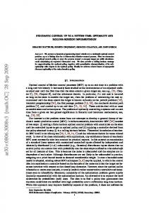
The SDALT algorithm [14] is a speed-up technique for DRegLC based on A∗ [11] and landmarks [9]. It is also based on DRegLC and works on the implicit product graph P . Different from DRegLC , SDALT uses an estimated lower bound of the distance to the target to guide the search more directly toward the target. More precisely, it employs a key k(v, s) = dr (v, s) + π(v, s) where dr (v, s) is the tentative distance label from (r, s0 ) to (v, s) and the potential function π : (V × S) → R gives an under-estimation of the distance from (v, s) to (t, s), s ∈ F0 . At every iteration, the algorithm selects the node (v, s) with the smallest key k(v, s). Intuitively, nodes which are close to the shortest estimated path between the source and the target node are explored first. So the closer π(v, s) is to the actual remaining distance, the faster the algorithm will find the target. It can be shown (see [12]) that SDALT is equivalent to DRegLC on a product graph with reduced arc costs cπ(v,sv )(w,sw )l = cvwl − π(v, sv ) + π(w, sw ). DRegLC is based on Dijkstra’s algorithm which works only for non-negative arc costs, so not all potential functions can be used. A potential function π is feasible, if cπ(v,sv )(w,sw )l is non-negative for all (v, w, l) ∈ A. Note that, if π 0 and π 00 are feasible potential functions, then max(π 0 , π 00 ) is a feasible potential function [9]. Tight bounds can be produced by using landmarks and the triangle inequality [9]. The main idea is to select a small set of nodes ` ∈ L ⊂ V (also called landmarks), appropriately spread over the network, and pre-compute all distances of shortest paths between the landmarks and any other node. By using these landmark distances and the triangle inequality, lower bounds on the distances between any two nodes can be derived. Finding good landmarks is difficult and several heuristics exist [9, 10]. SDALT applies these concepts to speed-up DRegLC on P by using the following potential function (see also Figure 1): [ π(v, s) = max {d0 (`, t, s) − d0 (`, v, s), d0 (v, `, s) − d0 (t, `, s), 0} (1) `∈L 0
d (i, j, s) denotes the constrained landmark distance, which is the travel time on the shortest path from (i, s) to (j, s0 ) for some s0 ∈ F0 constrained by the regular language Li→j . Here lies the major conceptual difference between SDALT and s uniALT. Differently from uniALT, SDALT does not use Dijkstra’s algorithm to determine landmark distances, but it uses the DRegLC algorithm instead. This way, it is possible to constrain the landmark distance calculation by some regular languages which is derived from L0 . Thus SDALT is able to already consider the constraints given by L0 during the preprocessing phase. Note that d0 (v, t, s) is constrained by
d0 (`, t, s), Ls`→t
d0 (v, `, s), Lv→` s
` d0 (`, v, s), Ls`→v
`
v
t d0 (v, t, s), Lv→t s
v
t
d0 (t, `, s), Lst→`
d0 (v, t, s), Lv→t s
Fig. 1: Landmark distances for SDALT
Lv→t = Ls0 . Ls0 is equal to L0 except that the initial state of A0 is replaced by s. s Intuitively Ls0 represents the constraints of L0 to be considered for the remaining portion of the shortest path from an arbitrary node (v, s) to the target. In [14] three methods, (bas), (adv), and (spe) have been presented on how to choose L`→t , L`→v , Lv→` , Lt→` used to constrain the calculation of d0 (`, t, s), s s s s 0 0 0 d (`, v, s), d (v, `, s), d (t, `, s) in such a way that the resulting potential function (Equation 1) results feasible and provides correct lower bounds. They are based on Proposition 1. Note that the concatenation of two regular languages L1 and L2 is the regular language L3 = L1 ◦ L2 = {v ◦ w|(v, w) ∈ L1 × L2 }. E.g., if L1 = {a, b} and L1 = {c, d} then L1 ◦ L2 = L3 = {ac, ad, bc, bd}. , then d0 (`, t, s) − ⊆ L`→t ◦ Lv→t Proposition 1 ([14]). For all s ∈ S, if L`→v s s s 0 0 v→t ⊆ Lv→` d (`, v, s) is a lower bound for the distance d (v, t, s). Equally, if Ls ◦Lt→` s s 0 0 0 then d (v, `, s) − d (t, `, s) is a lower bound for d (v, t, s).
4
Label Correcting State Dependent uniALT: lcSDALT
SDALT works correctly only if reduced arc costs are non-negative. It turns out, however, that by violating this condition often tighter lower bounds can be produced. This compensates, at least in our scenario, the additional computational effort required to remedy the disturbing effects of the use of negative reduced costs on the underlying Dijkstra’s algorithm and in addition results in shorter query times and lower memory requirements. This is why we propose a variation of SDALT, which can handle negative reduced costs. The major impact of this is that settled nodes may be re-inserted into the priority queue for re-examination (correction). In our setting, the number of arcs with non-negative reduced arc costs is limited and we can prove that the algorithm may stop once the target node is extracted from the priority queue. We name the new algorithm Label Correcting State Dependent uniALT (lcSDALT). Note that here label refers to the distance label of the algorithm and not to the labels on arcs. 4.1
Query
The algorithm lcSDALT is similar to DRegLC and uniALT. As priority queue Q we use a binary heap. The pseudo-code in figure 2 works as follows: the algorithm maintains, for every visited node (v, s) in the product graph P , a tentative distance label dr (v, s) and a parent node p(v, s). It starts by computing the potential for the start node (r, s0 ) and by inserting into Q (line 3). At every iteration, the algorithm
1 function SDALT_Lcor(G,r,t,τstart ,L0 ) 2 dr (v, s):= ∞, p(v, s):=-1, πv,s := 0, ∀(v, s) ∈ V × S 3 path_found:= false, dr (r, s0 ):= 0, k(r, s0 ):= π(r, s0 ), p(r, s0 ):= -1 4 insert (r, s0 ) in priority queue Q 5 while Q is not empty: 6 extract (v, s) with smallest key k from Q 7 if v == t and s ∈ F0 : 8 path_found:= true, break 9 for each (w, s0 ) s.t. (v, w, l) ∈ A ∧ s0 ∈ δ(l, s): 10 dtmp := dr (v, s) + cvwl (τstart + dr (v, s)) //time-dependency 11 if dtmp < dr (w, s0 ): 0 0 12 p(w, s ):= (v, s), dr (w, s ):= dtmp 14 if (w, s0 ) not in Q and never visited: //insert 15 πw,s0 := π(w, s0 ) 0 0 16 k(w, s ):= dr (w, s ) + πw,s0 17 insert (w, s0 ) in Q 18 elif (w, s0 ) not in Q: //re-insert 19 k(w, s0 ):= dr (w, s0 ) + πw,s0 20 insert (w, s0 ) in Q 21 else: //decrease 22 k(w, s0 ):= dr (w, s0 ) + πw,s0 0 23 decreaseKey w, s in Q 24 end for 25 end while
Fig. 2: Pseudo-code lcSDALT
extracts the node (v, s) in Q with the smallest key (the node is settled) and relaxes all outgoing arcs (line 9), i.e. checking and possibly updating the key and distance label for every node (w, s0 ) where s0 ∈ δ(l, s). More precisely, a new temporary distance label dtmp = dr (v, s) + cvwl (τstart + dr (v, s)) is compared to the currently assigned distance label (lines 10). If it is smaller, it either inserts or re-inserts node (w, s0 ) into the priority queue or decreases its key (line 14, 18, 21). Note that it is necessary to calculate the potential of a node (w, s0 ) only the first time it is visited. The cost of arc (v, w, l) might be time-dependent and thus has to be evaluated for time τstart + dr (v, s). The algorithm terminates when a node (t, s) with s ∈ F0 is settled. The resulting shortest path can be produced by following the parent nodes backward starting from node (t, s). Correctness The algorihtm lcSDALT is based on DRegLC and uniALT. It suffices to prove that when the target node (t, s0 ), s0 ∈ F0 is extracted from the priority queue the algorithm can stop (see Lemma 1 and Proposition 2). Note that π(t, s0 ) = 0, that d∗r (v, s) is the distance of the shortest path from (r, s0 ) to (v, s), and that there are no negative cycles as arc costs and potentials are always non-negative. Lemma 1. The priority queue always contains a node (i, s0 ) with key k(i, s0 ) = d∗r (i, s0 ) + π(i, s0 ) and which belongs to the shortest path from (r, s0 ) to (t, s00 ) where s00 ∈ F0 , s0 ∈ S. Proposition 2. If a solution exists, lcSDALT finds the shortest path. Proof. Let us suppose that a node (t, s), where s ∈ F0 , is extracted from the priority queue but its distance label is not optimal, so dr (t, s) 6= d∗r (t, s). Node (t, s) has key k(t, sf ) = dr (t, sf ) + π(t, s) 6= d∗r (t, s). By Lemma 1, this means that there exists
some node (i, s0 ) in the priority queue on the shortest path from (r, s0 ) to (t, s) which has not been settled because its key k(i, s0 ) > k(t, s). This means k(i, s0 ) = d∗r (i, s0 ) + π(i, s0 ) > dr (t, s) + π(t, s) = k(t, s), which is a contradiction. t u Complexity Complexity of DRegLC , SDALT as well as lcSDALT when a feasible potential function is used is equal to the complexity of the Dijkstra’s algorithm on the product graph P which is O(m log n) where m = |A||S|2 and n = |V ||S| are the number of arcs and nodes of P . If the potential function is non-feasible the key of a node extracted from the priority queue could not be minimal, hence already extracted nodes might have to be re-inserted into the priority queue at a later point (line 18-20) and re-examined (corrected). The algorithm lcSDALT can handle this but in this case its complexity is similar to the complexity of the Bellman-Ford algorithm (plus the time needed to manage the priority queue): O(mn log n). 4.2
Constrained landmark distances
For calculating the distance bounds for a generic node (v, s) of P , we give three procedures to determine the regular languages L`→t , L`→v , Lv→` , Lt→` which are s s s s used to constrain the landmark distance calculation (see Table 1). The languages produced by procedure 1 allows every combination of labels in Σ0 . The language produced by procedure 2 is similar but depends on the state s of the node (v, s). It allows every combination of labels in Σ0 except those labels for which there is no longer any transition between states which are reachable from s. Procedure 3 is the trickiest and produces four distinct languages for a node (v, s) of P . Ls`→t is determined in such a way that all constraints given by A0 on shortest paths considers only those which pass by a node (v, s) on A0 will be considered. Lv→` s constraints that apply to paths starting from (v, s) to a final node. Ls`→v and Lt→` s are derived in such a way that they put as few constraints as possible on the distance calculation but assure that Proposition 1 is valid. Consider, e.g., a transportation network. The procedures are based on the intuition that fast transportation modes which are excluded by L0 should also not be used to calculate the bounds. Also, if there are constraints which infer a major detour from the unconstrained shortest path, this detour should also be considered by the landmark distance calculation. In [14] these procedures have been used with SDALT to produce three methods which assure that reduced costs are always non-negative; a basic method (bas) which applies procedure 1 to all nodes (v, s) of P ; an advanced method (adv) which applies procedure 2 to all nodes and uses a slightly modified potential function; a specific method (spe) which applies procedure 3 to all nodes. These methods can also be used with lcSDALT. In the following we will present two new methods which can only be used with lcSDALT, as reduced costs may be negative: an adapted version of (adv) which we will call (advlc ) and a new method (mixlc ). (advlc ) Equally to (adv), this method applies procedure 2 to all nodes (v, s) of P . Differently to (adv) it uses Equation 1 as potential function and thereby considerably reduces the number of potentials to be calculated. (mixlc ) The method (spe) applies the regular languages constructed by applying procedure 3 for each state of L0 . This is space-consuming and bounds for nodes
proc. regular language and/or NFA 1 Lv→` = Lt→` = Ls`→v = Ls`→t = Lproc1 = {Σ0∗ } s s Lproc1 : Aproc1 = ({s}, Σ0 , δ : {s} × Σ0 → {s}, s, {s}) − → 2 Lv→` = Lt→` = Ls`→v = Ls`→t = Lproc2,s = { Σ (s, A0 )∗ } s s − → Lproc2,s : Aproc2,s = ({s}, Σ (s, A0 ), δ : {s} × Σ(s, A0 ) → {s}, s, {s}) ← − ← − 3 L`→v : A`→v = (S = S (s, A0 ), Σ = Σ (s, A0 ), δ0 |S×Σ ), s, {s}) s s ← − − → L`→t : A`→t = (S = S (s, A0 ) ∪ S (s, A0 ), s s ← − − → Σ = Σ (s, A0 ) ∪ Σ (s, A0 ), δ0 |S×Σ , s, F0 ∩ S) − → − → v→` Lv→` : A = (S = S (s, A0 ), Σ = Σ (s, A0 ), δ0 |S×Σ ), s, F0 ∩ S) s s T − → Lt→` : At→` = ({s}, Σ = s ∈ F0 ∩ S (s, A0 ){l ∈ Σ0 : ∃δ0 (s, l) = {s}}, s s δ : s × Σ = {s}, s, {s})
Table 1: With reference to a generic RegLCSP where the SP is constrained by regular language L0 (A0 = (S0 , Σ0 , δ0 , s0 , F0 )) the table shows three procedures to determine the regular language to constrain the distance calculation for a generic node (n, s) of the product graph P .
with certain states may be worse than those produced by procedure 2. This is why we introduce a more flexible new method (mixlc ) which provides the possibility to freely choose for each state between the application of procedure 2 or procedure 3. This also often gives a trade-off between memory requirements and performance improvement. To find the desired calibration for a given L0 and to determine when to use procedure 2 or procedure 3 some testing is necessary.
Memory requirements and time-dependency Memory requirements to hold preprocessing data for (advlc ) grow linearly in respect to |L| × |V | × |S|. (mixlc ) may require in the worst case up to four times more space than (advlc ). Similar to D, DRegLC and also lcSDALT can easily be adapted to the time-dependent scenario by selecting landmarks and calculating landmark distances by using the minimum weight cost function cijl = minτ cijl (τ ). Indeed, potentials stay valid as long as arc weights only increase and do not drop below a minimal value [2, 6]. 4.3
Experimental Results
The algorithm lcSDALT is implemented in C++ and compiled with GCC 4.1. A binary heap is used as priority queue. Similar to the basic version of uniALT [16], periodical additions of landmarks (max 6 landmark) take place. Experiments are run on a Intel Xeon, clocked at 2.6 Ghz, with 16 GB of RAM. The multi-modal transportation network is based on road and public transportation data of the French region Ile-de-France. It consists of five layers: private bike, rental bike, walking, car and public transportation. Each layer is connected to the walking layer through transfer arcs which model the time needed to transfer from one layer to another (e.g., the time needed to unchain and mount a bike). Each arc has exactly one associated label, e.g. f for arcs representing foot paths, ptr for train
f
f
b s0
t
s1
t
s2
L0 : f ∗ |(f ∗ tb∗ tf ∗ )
(a) A0 : Automaton allows walking (f ) and biking (b). Once the bike is discarded (state s2 ) it may not be used again. S0 = {s0 , s1 , s2 }, initial state s0 , F = {s0 , s2 }, Σ0 = {f, b, t}. (bas)
(adv)
(b) A0 expressed as a regular expression. The vertical bar | represents the boolean ’or’ and the asterisk ∗ indicates that there are zero or more of the preceding element.
(mix)
(spe) f s0
L`→v s 0
bf t
f s0
L`→t s 0
t
s0
(b|f |t)∗
f
L`→v = L`→t s s 2
f s0
f∗
t
t
s1
s0
f ∗ |(f ∗ tb∗ tf ∗ )
f ∗ tb∗
f
b t
s2
b s0
1
2
s1
f
L`→v s1 L`→t s
f∗
f
b
s1
t
s2
f ∗ tb∗ tf ∗
Fig. 3: Example of a regular language L0 (scenario A) and its representation as an automaton (3a) and regular expression (3b). The table lists the languages used to constrain the landmark distance calculation by applying (bas), (adv), (mix), and ∗ `→v (spe). E.g., for (adv): L`→v = Ls`→t = L`→v = L`→t = Ls`→t : f ∗. s0 s1 s1 : (b|f |t) , Ls2 0 2
tracks, ctoll for toll roads. The graph consists off circa 4.1mil arcs and 1.2mil nodes. Dimensions of the graph and a list off all used labels are given in Table 2. Data of the public transportation network has been provided by STIF4 . It includes geographical information, as well as timetable data on bus lines, tramways, subways and regional trains. Our model is similar to the one presented in [18]. Data for the car layer is based on road and traffic information provided by Mediamobile5 . Arc labels and travel time are set according to the road type. Circa 15% of the road arcs have a time-dependent cost function to represent changing traffic conditions throughout the day. Transfers from the car layer to the walking layer are possible at uniformly distributed transfers arcs. The walking as well as the private and rental bike layers are based on road data (walking paths, cycle paths, etc.) extracted from geographical data freely available from OpenStreetMap. Arc cost equals walking or biking time. Arcs are replicated and inserted in each of the layers if both walking and biking are possible. The rental bike layer includes only arcs in the area around the city of Paris, where the rental bike service6 is available. Bike rental stations serve as connection points between the walking layer and the rental bike layer as rental bikes have to be picked up and returned at bike rental stations. The private bike layer is connected to the walking layer at common street intersections. In addition, 4 5 6
Syndicat des Transports IdF, www.stif.info, data for scientific use (01/12/2010) www.v-trafic.fr, www.mediamobile.fr V´elib’, www.velib.paris.fr
layer nodes walking 275 606 public trans- 109 922 portation
arcs labels 751 144 f (all arcs except 20 arcs with label z) 292 113 pb (bus, 72 512 arcs), pm (metro, 1 746), pr (tram, 1 746), pt (train, 8 309), ptc (connection between stations, 32 490), ptw (walking station intern, 176 790), time-dependent 82 833 250 206 583 186 b 38 097 83 928 v 613 972 1 273 170 ctoll (toll roads, 3 784), cfast (fast roads, 16 502), cpav (paved roads except toll and fast roads, 1 212 957), cunpav (unpaved roads, 27 979), time-dependent 188 197 1 107 457 t (walking↔private bike 493 601, walking↔rental bike 2 404, walking↔car 572 604, walking↔public transportation 38 848) 1 287 803 4 095 971 time-dependent arcs 271 030 (7 687 204 Time Points)
private bike rental bike car
transfers Tot
Table 2: Dimensions of the graph
f ppc tvz
f ppc tv pb pt pw
pc
s1 f
t s0 t s4
cfast cpav
f
pb pt pw
s0
t
t
t
s3
s2
f
s2
p
s2
s3 ft
t
t t s1
t
z
s1
t
s4
s0
bf tz
bf t ft
s3
z
s4
t b
b s5
t f vt
(a) Scenario B
bf t s0
f tv bf tz z
s1
(b) Scenarios C and E
ft cf t
cf tz s5
z
s6
(c) Scenario D
Fig. 4: Instances used for experimental evaluation. Note that labels pb pm pr pt pw have been substituted by p and ctoll cfast cpav by c.
we introduced ten arcs with label z between nodes of the foot layer. They represent foot paths close to locations of interest, and are used to simulate the problem of reaching a target and in addition passing by any pharmacy, grocery shop, etc. We ran 500 test instances for five RegLCSP scenarios, see Figures 3a and 4. They have been chosen with the intention to represent real-world queries, which may arise when looking for constraint shortest paths on a multi-modal transportation network. Source node r, target node t, and start time τstart are picked at random. r and t always belong to the walking layer. We use 32 landmarks which are placed exclusively on the walking layer. Preprocessing for the different scenarios takes less than a minute. For each instance we compare running times of the different methods with DRegLC . See Table 3 for experimental results. time is the average running time in msec of the algorithm over 500 test instances. SettNo, reInsNo and calcPot give the average of the number of settled nodes, re-inserted nodes and calculated potentials. MaxSett gives the maximum number of settled nodes. For (mix)lc all states for which procedure 2 has been applied is given. For all other states procedure 3 has been used.
sce. method time speed-up settNo maxSett reInsNo nCalPot size proc 2 A DRegLC 238 1.0 296 656 986 292 0 (bas) 19 12.4 21 476 950 992 0 76 144 311 (adv) 18 13.6 10 930 684 296 0 129 020 622 (adv)lc 13 18.1 10 927 682 981 11 68 820 622 (spe) 62 3.9 45 548 202 382 0 272 174 1 244 (mix)lc 13 *18.9 11 034 254 259 19 74 544 933 s1 B DRegLC 624 1.0 610 375 1 487 766 0 (bas) 219 2.9 156 828 973 345 0 676 969 311 (adv) 190 3.3 51 258 346 549 0 2 295 030 1 866 (adv)lc 174 3.6 145 535 857 619 30 623 198 1 866 (spe) 237 2.6 176 766 667 125 0 543 388 2 177 (mix)lc 89 *7.0 60 053 350 237 87 343 585 1 244 s0 , s3 , s4 C DRegLC 630 1.0 658 738 1 785 747 0 (bas) 515 1.2 414 553 1 721 989 0 1 981 520 311 (adv) 338 1.9 158 193 977 793 0 2 437 770 933 (adv)lc 263 2.4 223 070 2 217 083 64 034 919 554 933 (spe) 238 2.7 156 739 929 544 0 633 859 1 866 (mix)lc 149 *4.2 91 917 499 646 1 064 674 115 1 244 s0 , s1 , s2 , s4 (mix)lc 161 3.9 97 119 620 991 2 564 686 516 933 s0 , s1 , s2 D DRegLC 1 722 1.0 1 248 060 3 085 428 0 (bas) 565 3.0 373 695 1 830 094 0 1 731 400 311 (adv) 695 2.5 352 969 1 557 331 0 3 297 090 1 244 (adv)lc 558 3.1 356 679 1 575 981 40 1 640 950 1 244 (spe) 476 3.6 337 849 1 791 504 0 734 068 2 488 (mix)lc 364 *4.7 221 631 1 278 208 48 953 802 2 177 s0 E DRegLC 764 1.0 795 822 1 458 519 0 (bas) 143 5.3 115 941 598 273 0 407 108 311 (adv) 119 6.4 115 941 598 273 0 411 869 311 (adv)lc 120 6.4 116 042 598 273 32 406 877 311 (spe) 25 30.3 27 532 216 389 0 109 125 622 (mix)lc 22 *34.4 23 607 145 308 608 85 776 933 s0
Table 3: Experimental results
4.4
Discussion of experimental results and conclusive remarks
The algorithm lcSDALT, by adopting the five methods (bas), (adv), (advlc ), (spe) and (mixlc ), in comparison to DRegLC , succeeds in directing the constrained shortest path search faster toward the target. (bas) works well in situations where L0 excludes a priori fast transportation modes (scenario A). (adv) gives a supplementary speedup in cases where initially allowed fast transportation modes are excluded from a later state on A0 onward. (spe) has a positive impact on running times for scenarios where the visit of some infrequent labels is imposed by L0 (E) or the use of fast transportation modes is somehow limited (B). Finally, the new methods (advlc ) and (mixlc ) prove to be very efficient. (advlc ) runs up to 20% faster than (adv) as it substantially reduces the number of calculated potentials, especially for larger automata. The extra flexibility provided by (mixlc ) often results in a reduction of running time (up to 50%) and a substantial reduction of memory space. Recent works on finding constrained shortest paths on multi-modal networks reported speed-ups of different orders of magnitude. They succeed in doing this by using contraction hierarchies and by either limiting the constraints which can be imposed on the shortest paths [19] or by identifying homogenous regions (arcs with the same label) of the network and by applying contractions only to those regions [7]. lcSDALT does not provide such speed-ups but proves to work consistently good even when considering more difficult constraints then the one considered in [19] and on a highly dis-homogenous graph. Also, time-dependent cost functions on arcs can
be easily incorporated. Therefore, lcSDALT seems a good ingredient to future more advances algorithms on multi-modal networks.
References 1. C. Barrett, K. Bisset, M. Holzer, G. Konjevod, M. Marathe, and D. Wagner. Engineering label-constrained shortest-path algorithms. Algorithmic Aspects in Information and Management, pages 27–37, 2008. 2. C. Barrett, K. Bisset, R. Jacob, G. Konjevod, and M. V. Marath. Classical and contemporary shortest path problems in road networks: Implementation and experimental analysis of the TRANSIMS router. Proc. ESA, pages 126–138, 2002. 3. C. Barrett, R. Jacob, and M. Marathe. Formal-Language-Constrained Path Problems. SIAM Journal on Computing, 30(3):809, 2000. 4. D. Delling, T. Pajor, and D. Wagner. Accelerating Multi-Modal Route Planning by Access-Nodes. Algorithms-ESA 2009, 2, 2009. 5. D. Delling, P. Sanders, D. Schultes, and D. Wagner. Engineering route planning algorithms. Algorithmics of large and complex networks, 2:117–139, 2009. 6. D. Delling and D. Wagner. Time-Dependent Route Planning. Online, 2:207–230, 2009. 7. J. Dibbelt, T. Pajor, and D. Wagner. User-Constrained Multi-Modal Route Planning. In Proceedings of the 14th Workshop on Algorithm Engineering and Experiments (ALENEX’12). SIAM, 2012. 8. E. W. Dijkstra. A note on two problems in connexion with graphs. Numerische Mathematik, 1(1):269–271, Dec. 1959. 9. A. V. Goldberg and C. Harrelson. Computing the shortest path: A search meets graph theory. In Proceedings of the 16th annual ACM-SIAM Symposium on Discrete algorithms, pages 156–165. SIAM, 2005. 10. A. V. Goldberg and R. Werneck. Computing point-to-point shortest paths from external memory. US Patent App. 11/115,558, 2005. 11. P. Hart, N. Nilsson, and B. Raphael. A Formal Basis for the Heuristic Determination of Minimum Cost Paths. IEEE Transactions on Systems Science and Cybernetics, 4(2):100–107, 1968. 12. T. Ikeda, H. Imai, S. Nishimura, H. Shimoura, T. Hashimoto, K. Tenmoku, and K. Mitoh. A fast algorithm for finding better routes by AI search techniques. IEEE, 1994. 13. D. Kaufman and R. Smith. Fastest paths in time-dependent networks for intelligent vehicle-highway systems applications. Journal of Intelligent Transportation Systems, 1(1):1–11, 1993. 14. D. Kirchler, L. Liberti, T. Pajor, and R. Wolfler Calvo. UniALT for Regular Language Constrained Shortest Paths on a Multi-Modal Transportation Network. In ATMOS 2011, pages 64–75. Schloss Dagstuhl, 2011. 15. A. O. Mendelzon and P. T. Wood. Finding Regular Simple Paths in Graph Databases. SIAM Journal on Computing, 24(6):1235, 1995. 16. G. Nannicini, D. Delling, L. Liberti, and D. Schultes. Bidirectional A search for timedependent fast paths. Experimental Algorithms, 2(2):334–346, 2008. 17. A. Orda and R. Rom. Shortest-path and minimum-delay algorithms in networks with time-dependent edge-length. Journal of the ACM, 37(3):607–625, July 1990. 18. E. Pyrga, F. Schulz, D. Wagner, and C. Zaroliagis. Efficient models for timetable information in public transportation systems. Journal of Experimental Algorithmics, 12(2):1–39, June 2007. 19. M. Rice. Graph indexing of road networks for shortest path queries with label restrictions. Proceedings of the VLDB Endowment, pages 69–80, 2010. 20. J. Romeuf. Shortest path under rational constraint. Information processing letters, 28(5):245–248, 1988.
A
Proofs
Lemma 2. The priority queue always contains a node (i, s0 ) with key k(i, s0 ) = d∗r (i, s0 ) + π(i, s0 ) and which belongs to the shortest path from (r, s0 ) to (t, s00 ) where s00 ∈ F0 , s0 ∈ S. Proof. Let q ∗ = (p1 = (r, s0 ), . . . , pm = (t, s00 )) be the shortest path from (r, s0 ) to (t, s00 ) on P (constrained by L0 ). At the first step of the algorithm node p1 = (r, s0 ) is inserted in the priority queue with key k(r, s) = d∗r (r, s) + π(r, s) = π(r, s). When node pn with k(i, s) = d∗r (i, s) + π(i, s) for some n ∈ {1, . . . , m} is extracted from the priority queue, at least one new node pn+1 = (j, s0 ) with dr (j, s0 ) = d∗r (j, s0 ) = t u d∗r (i, s) + c(i,s)(j,s0 )l (τ ) is inserted in the queue by lines 14, 18, 21.
B
Suppressed figures
π=1 π = 15 r
5
π = 10 5 1
1
2
π=3 5
4
π=0 5
t
1 3 π=9
step 1 insert node r in Q with key 15 step 2 extract node r from Q and insert node 1 in Q with key 15 step 3 extract node 1 from Q and insert node 2 in Q with key 11 and insert node 3 in Q with key 15 step 4 extract node 2 from Q and insert node 4 in Q with key 18 step 5 extract node 3 from Q and insert node 2 in Q with key 8 step 6 extract node 2 from Q and decrease node 3 in Q with key 15 step 7 extract node 4 from Q and insert node t in Q with key 15 step 8 extract node t from Q and terminate
Fig. 5: Application of algorithm lcSDALT without constraints. Arc from node 1 to node 2 has negative reduced cost 5 + 1 − 10 = −4 and as a result node 2 is inserted twice in the priority queue (P).
method characteristics (advlc ) lcSDALT uses Equation 1, SDALT for (adv) must apply a modified potential function: πadv (v, s) = max{π(v, sx )|sx ∈ Ω(s, A0 )} (mixlc ) mixes procedures 2 and 3
Table 4: Characteristics of (advlc ) and (mixlc )
algo DRegLC std bas
regular language to constrain distance calculation Lt→` Lv→` Lt→` Lv→` s0 s0 s1 s1 no potential not constrained (f |b)∗
adv spe
(f |b)∗ f ∗ bf ∗
f∗ f∗ 1
f, 1
3
f, 1
f, 4
settled nodes on P (key in square brackets) all (r, s0 )[9], . . . all except (1, s0 ), (2, s0 ) (r, s0 )[10], (5, s1 )[10], (6, s1 )[10],(7, s1 )[11], (8, s1 )[11], (t, s1 )[11] (r, s0 )[10], (5, s1 )[10], (7, s1 )[11], (8, s1 )[11], (t, s1 )[11] (r, s0 )[11], (7, s1 )[11], (8, s1 )[11],(t, s1 )[11] 2
4
c, 1
f, 4 r
b, 3
5
f, 4
6
b, 3 f, 4
b, 3 7
f, 4
8
t
f, 9
l f
f 0
b
1
Fig. 6: Example showing the application of lcSDALT on a labeled graph. The shortest paths is constrained by the regular expression f ∗ bf ∗ (NFA on the right of the graph). The table shows the regular languages used to constrain the landmark distance calculation, as well as the search space. Optimal path: (r, s0 ), (9, s1 ), (10, s1 ), (t, s1 ). Node l is the landmark.
C
Further details for instances
Here we provide more information about the instances used for experimental evaluation. Note that labels pb pm pr pt pw have been substituted by p and ctoll cfast cpav by c. f
f
b t
s0
t
s1
s2
Fig. 7: Scenario A: The target may be reach be either walking or walking and taking a private bike. Once discarded, the bike may not be used again.
pb pt pw
pb pt pw pc
s1 f s0 t
t
t
t
s3
s2
t
t
t b
s4
s5
t
cfast cpav
f vt
Fig. 8: Scenario B: The target may be reached by walking or by using a private car (only paved and fast roads are allowed, no toll roads). The target may also be reached by private bike or/and by taking public transportation (no metro allowed). Maximal one change of public transportation vehicles is permitted. Once discarded the private car or private bike or left public transportation, the itinerary may be continued by walking or by taking a rental bike.
f s2
f s0
p t
t
t t s1 b
s3
s4 f tv
Fig. 9: Scenario C: The target may be reached by walking or by taking a private bike. Public transportation may be used once but without changing vehicles. Once left public transportation, the itinerary may be continued by walking or by taking a rental bike.
bf tz
bf t s0
z
s1
Fig. 10: Scenario E: At any point of the itinerary taking a private bike or walking is possible. An arc with label z has obligatorily to be visited. It may represent a street with a grocery shop, a post office, etc
f ppc tvz
f ppc tv
z
s1 ft s0
bf tz
bf t ft
s2
s3
ft cf t
z
s4
cf tz s5
z
s6
Fig. 11: Scenario D: An arc with label z has obligatorily to be visited. It may represent a street with a grocery shop, a post office, etc. Other than that either public transportation or private bike or private car may be used.