Yugoslav Journal of Operations Research 27 (2017), Number 1, 46–60 DOI: 10.2298/YJOR150624009T
EFFICIENT ALGORITHMS FOR THE REVERSE SHORTEST PATH PROBLEM ON TREES UNDER THE HAMMING DISTANCE Javad TAYYEBI* Department of Industrial Engineering, Birjand University of Technology, Birjand, Iran
[email protected],
[email protected] Massoud AMAN Department of Mathematics, Faculty of Mathematical Sciences and Statistic, University of Birjand, Birjand, Iran
[email protected]
Received: June 2015 / Accepted: May 2016 Abstract: Given a network G(V, A, c) and a collection of origin-destination pairs with prescribed values, the reverse shortest path problem is to modify the arc length vector c as little as possible under some bound constraints such that the shortest distance between each origin-destination pair is upper bounded by the corresponding prescribed value. It is known that the reverse shortest path problem is NP-hard even on trees when the arc length modifications are measured by the weighted sum-type Hamming distance. In this paper, we consider two special cases of this problem which are polynomially solvable. The first is the case with uniform lengths. It is shown that this case transforms to a minimum cost flow problem on an auxiliary network. An efficient algorithm is also proposed for solving this case under the unit sum-type Hamming distance. The second case considered is the problem without bound constraints. It is shown that this case is reduced to a minimum cut problem on a tree-like network. Therefore, both cases studied can be solved in strongly polynomial time. Keywords: Inverse problems, Shortest path problem, Hamming distance, Combinatorial algorithms. MSC: 90C27, 90C35, 05C85. * Corresponding author
J. Tayyebi, M. Aman / Efficient Algorithms for the Reverse Shortest Path Problem
47
1. INTRODUCTION Suppose that G(V, A, c) is a directed and connected network where V is the set of nodes, A is the set of arcs and c is the nonnegative arc length vector. Let S ⊆ V × V be a collection of origin-destination pairs (si , ti ), i = 1, . . . , k. The well-known shortest path problem is to find the shortest paths between each (si , ti ) ∈ S on G. This problem has a wide variety of applications in practice such as transportation systems, computer networks. It is also theoretically interested because there exists several efficient algorithms to solve the problem and furthermore, the problem arises frequently as a subproblem when solving many combinatorial and network optimization problems [1]. For any optimization problem, one can introduce some inverse problems. We refer readers to the survey paper [11] for more details on inverse optimization problems. Two general classes of the inverse shortest path problems are studied in the literature: the inverse shortest path (ISP) problem and the reverse shortest path (RSP) problem. The ISP problem is to adjust the arc lengths minimally such that each given path from si to ti becomes a shortest path. The RSP problem consists of modifying the arc lengths as little as possible so that the shortest distance between each pair (si , ti ) is upper bounded by a prescribed value di ≥ 0. The RSP problem is also called as ”the shortest path improvement problem” and ”the inverse shortest path lengths problem” by some authors [7, 16]. The inverse and reverse shortest path problems have attracted great attention due to its broad applications in practice such as the traffic modeling, the seismic tomography, and the design of computer networks [3, 4, 6, 10]. Zhang et. al [19] showed that the ISP problem is equivalent to solving a minimumweight circulation problem when the modifications are measured by the l1 norm. In [18], a column generation scheme is developed to solve the ISP problem under the l1 norm. Ahuja and Orlin [2] showed that the ISP problem under the l1 norm can be solved by solving a new shortest path problem. For the l∞ norm, they showed that the problem reduces to a minimum mean cycle problem. In [15], it is shown that all feasible solutions of the ISP problem form a polyhedral cone and the relationship between this problem and the minimum cut problem is discussed. Duin and Volgenant [8] proposed an efficient algorithm based on the binary search technique to solve the ISP problem under the bottleneck-type Hamming distance. In [12, 13], we extended their method to solve the inverse minimum cost flow problem and the inverse linear programming problem. The concept of the inverse optimization problems was introduced by Burton and Toint [3, 4]. They studied the RSP problem under the l2 norm and proposed a method based on nonlinear optimization techniques to solve the problem. In [5], it is shown that the RSP problem under the l2 norm is NP-hard. A similar result is obtained for the l1 norm in [7, 20] and also, efficient algorithms are proposed in some special cases. Fekete et. al [9] studied the complexity of obtaining a feasible solution to the RSP problem. They showed that it is intractable even in very restricted cases. The RSP problem under the weighted sum-type Hamming distance is formulated
48
J. Tayyebi, M. Aman / Efficient Algorithms for the Reverse Shortest Path Problem
as follows [16]: min
z=
X
w j H(c j , cˆ j )
e j ∈A
s.t.
dcˆ (si , ti ) ≤ di ∀(si , ti ) ∈ S, 0 ≤ cˆ j ≤ c j ∀e j ∈ A,
(1)
where dcˆ (si , ti ) is the length of the shortest path from si to ti with respect to the length vector cˆ ; H(c j , cˆ j ) is the Hamming distance between c j and cˆ j (i.e., H(c j , cˆ j ) = 0 if cˆ j = c j and H(c j , cˆ j ) = 1, otherwise); w j ≥ 0 is a penalty for modifying the length of each arc e j and di ≥ 0 is the prescribed distance for each origin-destination pair (si , ti ). Two cases of the problem (1) are proved to be NP-hard in [16]: • The RSP problem with a single origin in which c j = w j = 1 for every e j ∈ A: We call this problem as the RSP (URSP) problem with uniform data. • The RSP problem on trees with a single origin: This problem is referred to as the RSP (TRSP) problem on trees. The second result is interested because the RSP problem on trees under the l1 norm is polynomially solvable [20]. This is a reason why the behaviour of the RSP problem under the Hamming distances is different from that of the problem under norms. An alternative reason is that the Hamming distances unlike to norms are nonconvex and discontinuous. Therefore, the known approaches for norms cannot be applied for solving the RSP problem under the Hamming distances. As the RSP problem on trees under the sum-type Hamming distance is NP-hard, this aspect is worthwhile to further study special cases which the problem is polynomially solvable. In [17], the authors proposed polynomial-time algorithms to solve the problem under the unit Hamming distance on chain networks and star-tree networks. Then, they designed an efficient algorithm for solving the TRSP problem with a very special constraint on paths. In this article, we first consider the TRSP problem when c j = 1 for each e j ∈ A. It is shown that the problem transforms to an instance of the minimum cost flow problem due to the special form of its coefficient matrix. As a special case, we propose a simple algorithm to solve the problem that is in the intersection of the ULRSP and TRSP problems. We also consider the TRSP problem without nonnegativity constraints and show that the problem can be reduced to solving a minimum cut problem on a tree-like network. Figure 1 provides a diagram to compare the complexities of these problems. The rest of this article is organized as follows: Section 2 focuses on the TRSP problem with uniform lengths. Section 3 considers the TRSP problem with uniform penalties and uniform lengths. Section 4 discusses the RSP problem without nonnegativity restrictions. Section 5 presents some computational experiments of our proposed algorithms. Finally, some concluding remarks are given in Section 6.
J. Tayyebi, M. Aman / Efficient Algorithms for the Reverse Shortest Path Problem
49
Figure 1: Complexity of the RSP problem
2. REVERSE SHORTEST PATH PROBLEM ON TREES WITH UNIFORM LENGTHS Suppose that T(V, A) is a tree where V is the set of n nodes, A = {e1 , e2 , . . . , en−1 } is the set of arcs. In this section, we consider the TRSP problem when all arc lengths are equal to 1. The problem contains a single origin s and multiple destinations ti , i = 1, 2, . . . , k. We assume that T is a directed out-tree rooted at node s, i.e., the unique path in the tree from node s to every other node is a directed path. This problem can be formulated as follows: X min z = w j H(1, cˆ j ) (2a) e j ∈A
s.t.
X
cˆ j ≤ di
∀i = 1, . . . , k,
(2b)
e j ∈Pti
0 ≤ cˆ j ≤ 1
∀e j ∈ A,
(2c)
where Pti is the unique path from s to each destination node ti and the other parameters are defined as in the problem (1). Note that the problem (2) is feasible because cˆ = 0 is a feasible solution to the problem. In T, we denote the head node of each e j ∈ A as ve j . For every arc e j ∈ A, we denote the subtree of T rooted at ve j as Te j and the unique path from s to ve j by Pe j . Lemma 2.1. The problem (2) has a zero-one optimal solution.
50
J. Tayyebi, M. Aman / Efficient Algorithms for the Reverse Shortest Path Problem
Proof. Since the set of objective values of the problem is finite, the problem has at least one optimal solution cˆ∗ . Define the solution cˆ ∗∗ as follows: ( 1 cˆ∗j = 1, ∗∗ cˆ j = ∀e j ∈ A. 0 cˆ∗j , 1, We show that cˆ ∗∗ is also optimal to the problem (2). It is obvious that the objective values of both the solutions are the same because cˆ∗j , 1 if and only if cˆ∗∗j , 1 for each e j ∈ A. On the other hand, cˆ ∗∗ ≤ cˆ ∗ based on the definition of cˆ ∗∗ . This guarantees that cˆ ∗∗ is also feasible to the problem because X X cˆ∗j ≤ di ∀i = 1, 2, . . . , k. cˆ∗∗j ≤ e j ∈Pti
e j ∈Pti
Therefore, the problem has the zero-one optimal solution cˆ ∗∗ . By using Lemma 2.1, we can restrict our attention to zero-one solutions. Therefore, the problem is converted into the following problem: X X X min z = w j (1 − cˆ j ) = wj − w j cˆ j e j ∈A
s.t.
X
cˆ j ≤ di
e j ∈A
e j ∈A
∀i = 1, . . . , k,
e j ∈Pti
cˆ j = 0 or 1 ∀e j ∈ A, In matrix form, this problem is rewritten as min z = wˆc s.t. Bˆc ≤ d, cˆ ∈ {0, 1}n−1 ,
(3a) (3b) (3c)
where w = [−w1 , −w2 , . . . , −wn−1 ], d = [d1 , d2 , . . . , dk ] , cˆ = [ˆc1 , cˆ2 , . . . , cˆn−1 ] and B = (b1 , b2 , . . . , bn−1 ) is a k × (n − 1) matrix whose jth column is defined as follows: ( 1 e j ∈ Pti , bi j = ∀i = 1, 2, . . . , k. 0 e j < Pti , T
T
As an immediate consequence, we can assume that the prescribed values di are integral because the left-hand side of each constraint (3b) is an integer between 0 and [di ] for each zero-one feasible solution cˆ . We next show that 1’s of each column of the coefficient matrix B are consecutive if its rows are arranged in a special fashion. This result guarantees that the problem can transform to an instance of the minimum cost flow problem on an auxiliary network. Since each row of B corresponds to a destination node, it is sufficient to sort the destination nodes. The Depth-First-Search (DFS) algorithm is used to traverse nodes of T starting from the origin node s. Assume that D = {t1 , t2 , . . . , tk } is the set of destinations sorted in the order of their traversal by the DFS algorithm.
J. Tayyebi, M. Aman / Efficient Algorithms for the Reverse Shortest Path Problem
51
Theorem 2.2. 1’s of each column of the matrix B are consecutive whenever the constraints (3b) are arranged in the order of D. Proof. For each column bj , bi j = 1 if e j ∈ Pti . Equivalently, bi j = 1 if ti ∈ Te j . Since nodes of Te j are visited consecutively by the DFS algorithm, it follows that 1’s of b j are consecutive. Based on Theorem 2.2, we can transform the problem (3) into a minimum cost flow problem due to the special form of the coefficient matrix [1]. Let the constraints (3b) be arranged in the order of D. We first introduce a slack variable si for each constraint (3b) to bring it into an equality form and also, add a redundant equality constraint 0.ˆc = 0. Therefore, the problem has k + 1 equality constraints. We next subtract the ith constraint from the (i + 1)th constraint for each i = 1, 2, . . . , k. Suppose that B0 and d0 are the new coefficient matrix and the new right hand vector, respectively. Theorem 2.2 implies that B0 is a matrix whose each column has exactly one +1 and exactly one −1 (i.e., B0 is an incidence matrix). On the other P 0 hand, it can easily seen that k+1 i=1 di = 0. Therefore, the problem (3) is converted into the following equivalent problem: min s.t.
z =" wˆc# cˆ = d0 , B0 s
(4)
cˆ j = 0 or 1 ∀e j ∈ A, si ≥ 0
∀i ∈ {1, 2, . . . , k},
Note that the relaxation 0 ≤ cˆ ≤ 1 converts the problem into a minimum cost flow problem because B0 is an incidence matrix. Since each minimum cost flow problem with integral data has at least an optimal integer solution and most minimum cost flow algorithms obtain such the optimal solutions [1], we can use this relaxation. Therefore, the problem (3) reduces to an instance of the minimum cost flow problem on the auxiliary network G0 (V 0 , A0 , w, d0 ) which is defined as follows: • The node set is V 0 = {t1 , t2 , . . . , tk , tk+1 } where tk+1 corresponds to the redundant equality constraint 0.ˆc = 0. • The arc set is A0 = A ∪ {s1 , . . . , sk }. Each arc e j ∈ A emanates from tu and terminates at tv where u is the row corresponding to the first 1 of b j and v is the row corresponding to the first 0 of b j after u. Each arc si emanates from ti and terminates at ti+1 . • The cost of each arc e j is −w j and the cost of each arc si is zero. • The upper bound of each arc e j is 1 and each arc si has an infinite upper bound. • Node ti has a supply or demand equal to d0i = di −di−1 for each i ∈ {2, 3, . . . , k+ 1} and the supply of t1 is d1 ≥ 0.
52
J. Tayyebi, M. Aman / Efficient Algorithms for the Reverse Shortest Path Problem
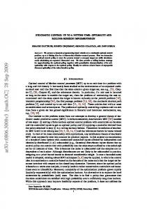
Figure 2: (a) A network G(V, A, w); (b) the auxiliary network G0 (V 0 , A0 , w, d0 )
We illustrate this transformation using an example. Example 2.3. Consider an instance of the problem (2) defined on the network shown in Figure 2.a. The coefficient matrix B is as follows: cˆ1 1 1 1
t1 t2 t3
B=
cˆ2 1 1 0
cˆ3 0 1 0
cˆ4 0 0 1
cˆ5 0 0 1
.
Note that rows of B are sorted by the DFS algorithm and hence, Theorem 2.2 holds. The new coefficient matrix is
B0 =
t1 t2 t3 t4
cˆ1 1 0 0 -1
cˆ2 1 0 -1 0
cˆ3 0 1 -1 0
cˆ4 0 0 1 -1
cˆ5 0 0 1 -1
s1 1 -1 0 0
s2 0 1 -1 0
s3 0 0 1 -1
.
The auxiliary network G0 is shown in Figure 2.b. By solving the minimum cost flow problem defined on G0 , we obtain the optimal solution cˆ2 = cˆ3 = cˆ5 = 1, cˆ1 = cˆ4 = s1 = s2 = s3 = 0, z = −1 − 3 − 5 = −9. Therefore, the optimal solution of the P problem (2)Pis to change only the cost of e1 and e4 from 1 to 0. Its objective value is 4 = j∈e j w j − w j cˆ j = 13 − 9. The auxiliary network contains k + 1 nodes and n + k − 1 arcs. One can use the enhanced capacity scaling algorithm to solve the associated minimum cost flow problem in O(n2 log k +nk log2 k) time [1]. Therefore, the problem (2) can be solved in the same time.
J. Tayyebi, M. Aman / Efficient Algorithms for the Reverse Shortest Path Problem
53
Remark 2.4. In the problem (2), we have assume that c j = 1 for each e j ∈ A. It is easy to see that this transformation is valid for the problem with uniform lengths, and not necessarily unit lengths. 3. REVERSE SHORTEST PATH PROBLEM ON TREES WITH UNIFORM PENALTIES AND UNIFORM LENGTHS In this section, we consider the TRSP problem when w j = c j = 1 for every e j ∈ A. The TRSP problem with uniform penalties and uniform lengths is simply convertible to this special case. Note that this problem is a special type of the problem (2) with unit penalties and consequently, it can be solved efficiently by the transformation stated in Section 2. However, we here present a simple algorithm to solve the problem with a better complexity. Similar to the problem (2), we can formulate the TRSP problem with unit penalties as well as unit lengths as follows: X min z = H(1, cˆ j ) e j ∈A
s.t.
X
cˆ j ≤ di
∀i = 1, . . . , k,
(5)
e j ∈Pti
0 ≤ cˆ j ≤ 1
∀e j ∈ A,
where the parameters are defined as in the problems (1) and (2). Based on Lemma 2.1, we restrict our attention to solutions cˆ with cˆ j = 0 or 1 for every e j ∈ A. Any such solution is determined by an arc set S ⊆ A as follows: ( 0 e j ∈ S, cˆ j = ∀e j ∈ A. (6) 1 e j ∈ A\S, A solution cˆ corresponding to S has the objective value equal to |S|. Our proposed algorithm begins with S = ∅ and checks whether or not the corresponding solution is feasible. If the solution is feasible, the algorithm terminates and otherwise, it goes to the next iteration by adding one arc eq to S. This process is repeated until a feasible solution is obtained. For a given set S, if the value X X X d0i = cˆ j − di = ( 0+ 1) − di = |Pti \S| − di e j ∈Pti
e j ∈Pti ∩S
e j ∈Pti \S
is nonpositive for each i = 1, 2, . . . , k, then the solution cˆ corresponding to S is feasible to the problem (5). In other words, the solution corresponding to S is feasible if S contains at least |Pti | − di elements of Pti for each i = 1, 2, . . . , k. Therefore, the problem (5) is reduced to the following problem: min |S|
(7)
S⊆A
s.t. d0i ≤ 0,
∀i = 1, 2, . . . , k.
54
J. Tayyebi, M. Aman / Efficient Algorithms for the Reverse Shortest Path Problem
For obtaining the optimal solution S to the problem (7), we put arcs closer to the origin s into S because such arcs belong to more sets Pti . For this purpose, we use the Breadth-First-Search algorithm to traverse arcs starting from the origin node s (see Algorithm 1). The set S obtained by Algorithm 1 has obviously the following property: if e j Input: A tree T(V, A), an origin node s and a collection of destination nodes ti , i = 1, 2, . . . , k, with nonnegative prescribed distances di . 2 Initialization: Apply the BFS algorithm to traverse the tree starting from the origin s. Suppose that A = {e1 , e2 , . . . , en−1 } is the sorted set of arcs in the order of their appearance. 3 S = ∅. 4 j = 1. 5 For j=1 to n-1 do 6 For i=1 to k do 7 If e j ∈ Pti and d0i > 0, then S = S ∪ {e j }. 8 For l=1 to k do 9 If e j ∈ Ptl , then d0 (l) = d0 (l) − 1. 10 Output The solution corresponding to S defined by (6) is optimal to the problem (5) with the optimal objective value |S|. Algorithm 1: Reverse problem with uniform penalties and uniform lengths 1
belongs to S, then each arc on the unique path from the origin s to e j also belongs to S. The following lemma guarantees the existence of an optimal solution with this property. Lemma 3.1. There exists an optimal solution S∗ to the problem (7) so that if e j ∈ S∗ , then el ∈ S∗ for each el ∈ Pe j . Proof. The problem (7) is feasible because S = A is a feasible solution to the problem. Since the problem (7) has a finite number of feasible solutions, it follows that the problem has at least an optimal solution. Suppose that S∗ is an optimal solution to the problem. If S∗ does not satisfy the desired property, then e j ∈ S∗ and el < S∗ for some e j ∈ A and some el ∈ Pe j . Define S¯ = (S∗ \{e j }) ∪ {el }. The relation e j ∈ Tel together with the feasibility of S∗ guarantee that S¯ is feasible to ¯ By the problem (7). Therefore, S¯ is also an optimal solution because |S∗ | = |S|. ¯ repeating this process, we can obtain an optimal solution S satisfying the desired property. Theorem 3.2. Algorithm 1 solves the problem (5) in O(nk) time. Proof. Suppose that cˆ is the solution corresponding to the set S obtained by the algorithm. For proving the correctness of Algorithm 1, we show that cˆ is feasible and optimal to the problem (5). Suppose that cˆ is not feasible by contradiction. Then, there exists some index i0 ∈ {1, 2, . . . , k} such that d0i0 > 0. Consequently,
J. Tayyebi, M. Aman / Efficient Algorithms for the Reverse Shortest Path Problem
55
|S ∩ Pti0 | < |Pti0 |. This implies that there exists at least one arc e j0 belonging to Pti0 \S. This contradicts the process of line 7 of Algorithm 1 because e j0 < S while e j0 ∈ Pti0 with d0i0 > 0. Assume that S∗ is an optimal solution of the problem (7) satisfying the conditions of Lemma 3.1. Suppose that S is the set obtained by Algorithm 1 and |S| > |S∗ | by contradiction. Then, S\S∗ , ∅. Select one arc e j0 ∈ S\S∗ with the property that S ∩ Te j0 = ∅. Based on Lemma 3.1, S∗ ∩ Te j0 = ∅. Hence, d0i = |Pti \S| − di < |Pti \S∗ | − di ≤ 0
∀ti ∈ Te j0 .
(8)
Consider the iteration that e j0 is added to S. In this iteration, d0i0 = |Pti0 \S| − di0 > 0 for some ti0 ∈ Te j0 . Adding e j0 to S decreases d0i0 by one unit. In the next iterations, d0i0 remains unchanged because S ∩ Te j0 = ∅. Therefore, d0i0 is nonnegative which contradicts (8). Now, we analyze the complexity of Algorithm 1. The number of iterations is n − 1 because the algorithm examines one arc in each iteration. We show that line 6 of Algorithm 1 can be done in O(k) time. This implies that the complexity of Algorithm 1 is O(kn). For each arc e j ∈ A, suppose that the accessible list L(e j ) is the set of destination nodes ti so that e j ∈ Pti . The algorithm maintains each accessible list L(e j ) as a linked list. In each iteration, an accessible list is traversed to check the existence of an index i ∈ {1, 2, . . . , k} with e j ∈ Pti and d0i > 0. When arc e j is added to S, d0i is decreased by 1 for each ti ∈ L(e j ). Both these operations require at most O(k) time. This completes the proof. Example 3.3. Consider the problem (5) defined on the network shown in Figure 2.a. Algorithm 1 gives us the optimal solution corresponding to S = {e1 , e4 }. 4. REVERSE PROBLEM WITHOUT NONNEGATIVITY RESTRICTIONS In this section, we consider the TRSP problem without nonnegativity restrictions, and show that the problem is transformable to a minimum cut problem on a tree-like network. Consequently, it can be solved in strongly polynomial time. For a given tree T(V, A) with length vector c, the problem (1) on trees without nonnegativity restrictions is stated formally as follows: X min z = w j H(c j , cˆ j ) e j ∈A
s.t.
X
cˆ j ≤ di
∀i = 1, . . . , k,
(9)
e j ∈Pti
cˆ j ≤ c j
∀e j ∈ A,
where the parameters are defined as in the problems (1) and (2). Remark 4.1. In the previous sections, we have assumed that the arc lengths and the prescribed distances are nonnegative. Here, we drop this assumption.
56
J. Tayyebi, M. Aman / Efficient Algorithms for the Reverse Shortest Path Problem
Suppose that V 0 is the subset of {1, 2, . . . , k} so that i ∈ V 0 if and only if d00 = i P ¯ ¯ ¯ ¯ in the e j ∈Pti c j − di is positive. We construct the tree-like network G(V, A, w) following manner. • The node set V¯ is V ∪ {t}. • G¯ contains the same arcs of T plus additional arcs (ti , t), called artificial arcs, for each i ∈ V 0 , i.e., A¯ = A ∪ {(ti , t) : i ∈ V 0 }. P • Each arc e j ∈ A has a capacity w¯ j equal to w j and a fixed capacity W = e j ∈A w j is associated with each artificial arc. ¯ V, ¯ w). ¯ A, ¯ Obviously, C∗ has not any Suppose that C∗ is a minimum s − t cut of G( ∗ artificial arc. Consider the solution cˆ defined by ( cj e j < C∗ , cˆ∗j = c − max ∀e j ∈ A. (10) 00 {d } e ∈ C∗ , j
ti ∈Te j
j
i
We show that cˆ ∗ is an optimal solution to the problem (9). First, note that there exists at least one destination ti ∈ Te j with d00 > 0 for each e j ∈ C∗ . If not, we i ∗ ∗ can remove e j from C and however, C remains an s − t cut which contradicts to ∗ the definition of a cut. that P This implies P the objective value of cˆ is equal to the ∗ ∗ capacity of C , i.e., e j ∈A w j H(c j , cˆ j ) = e j ∈C∗ w j . The fact that there exists an arc e ji belonging to C∗ for each i ∈ V 0 guarantees that cˆ ∗ is feasible because X X c j − max{d00 cˆ∗j ≤ l } e j ∈Pti
e j ∈Pti
≤
X
tl ∈Te j
i
c j − d00 i = di
∀i ∈ V 0 .
e j ∈Pti ∗
Suppose that cˆ isPnot optimal by contradiction. Then, there exists a feasible P solution cˆ 0 so that e j ∈A w j H(c j , cˆ0j ) < e j ∈C∗ w j . Let C0 be the set of modified arcs of cˆ 0 , i.e., C0 = {e j ∈ A : cˆ0j , c j }. It is easy to see that C0 separates s and t. Therefore, C0 contains an s − t cut whose capacity is less than that of the cut C∗ . This leads to a contradiction. We have thus established the following result. ¯ V, ¯ w), ¯ A, ¯ then cˆ ∗ defined by (10) is an Lemma 4.2. If C∗ is a minimum s − t cut of G( optimal solution to the problem (9). Now we are ready to state the proposed algorithm (see Algorithm 2) for solving the problem (9). Theorem 4.3. Algorithm 2 solves the problem (9) in O(n) time. Proof. The correctness of Algorithm 2 is immediate by Lemma 4.2. We analyze its complexity. Obviously, the bottleneck operation is to find a minimum cut on the ¯ This can be done in linear time by solving the corresponding tree-like network G. maximum flow problem (refer to Theorem 2 of [14]). Therefore, Algorithm 2 can solve the problem (9) in linear time.
J. Tayyebi, M. Aman / Efficient Algorithms for the Reverse Shortest Path Problem 1
2 3 4 5 6 7 8 9 10 11 12 13
57
Input: A tree T(V, A) with length vector c and penalty vector w, an origin node s and a collection of destination nodes ti , i = 1, 2, . . . , k, with prescribed distances di . P For i ∈ {1, 2, . . . , t} do d00 = e j ∈Pt c j − di . i i flag= true. For i ∈ {1, 2, . . . , t} do If d00 > 0 then flag=false. i If flag==true then cˆ ∗ = c and stop else V 0 = {i : d00 > 0}. i ¯ V, ¯ w) ¯ A, ¯ in the following manner: Construct the tree-like network G( V¯ = V ∪ {t}. A¯ = A ∪ {(ti , t) : i ∈ V 0 }. P If e j ∈ A then w¯ j = w j else w¯ j = e j ∈A w j . ¯ V, ¯ w). ¯ A, ¯ Find a minimum s − t cut C∗ of G( ∗ ∗ Obtain cˆ by (10) using C . Output: cˆ ∗ is an optimal solution to the problem (9). Algorithm 2: Reverse problem without nonnegativity restrictions
5. COMPUTATIONAL EXPERIMENTS In this section, we have conducted a computational study to observe the performance of Algorithms 1 and 2. The following computational tools were used to develop algorithms: Python 2.7.5, Matplotlib 1.3.1 and NetworkX 1.8.1. All computational experiments were conducted on a 32-bit Windows 7 with Processor Intel(R) Core(TM) i5 − 3210M CPU @2.50GHz and 4 GB of RAM. For computational experiments, we first generate a random tree with n nodes. We suppose that trees are rooted in an origin node s and their arcs are orientated such that a unique path exists from s to each other nodes. In generated instances, we use random data generated using a uniform random distribution as follows: ci j ∼ U(1, n) ∀(i, j) ∈ A, wi j ∼ U(1, n) ∀(i, j) ∈ A, di ∼ U(1, n) ∀i ∈ V. We count the average number of modified arcs and calculate average CPU time on a series of instances. We have tested the algorithms on five classes of networks which differ from the number of nodes, varying from 10 to 1000. There are 100 random instances generated for each class of networks. Tables 1 and 2 present average performance statistics of Algorithms 1 and 2, respectively. The running times of Algorithms 1 and 2 grow linearly as the size of instance increases. It is remarkable that the number of modified arcs in the reverse problems with uniform data increases faster than that in the unconstrained reverse problems. This is a reasonable result because in the unconstrained problem, arc costs can
58
J. Tayyebi, M. Aman / Efficient Algorithms for the Reverse Shortest Path Problem Table 1: Average performance statistics of Algorithm 1
Number of nodes
Average running time (second)
Average number of modified arcs
10 50 100 500 1000
0.0065 0.0083 0.0139 0.0413 0.1004
1.88 8.92 15.28 40.65 73.6
Table 2: Average performance statistics of Algorithm 2
Number of nodes
Average running time (second)
Average number of modified arcs
10 50 100 500 1000
0.0050 0.0090 0.0182 0.1133 0.2102
1.87 2.1 2.22 2.28 2.30
be decreased in any arbitrary amount and consequently, the lesser number of modifications can satisfy the constraints (2b). As a special case of trees, we perform experiments on star-tree networks G where any two origin-destination paths of G have no common arcs [17]. Throughout experiments, we assume that the origin node s is a leaf of G, i.e., one node with degree 1. Table 3 presents experimental results. As seen in Table 3, Algorithm 2 often needs to modify capacity of one arc for solving the problem. This arc is the one with least penalty among all the arcs on the path from s to a node whose degree is greater than 2. 6. CONCLUSION It is known that the reverse shortest path problem on trees under the sum-type Hamming distance is NP-hard [16]. In this article, we studied the special cases of the problem which are polynomially solvable. First, we considered the case with uniform lengths and showed that this problem can be transformed to a minimum
Table 3: Average performance statistics of Algorithms 1 and 2 for star-tree networks
Number of nodes
Average running time (second)
Average number of modified arcs
10 50 100 500 1000
Algorithm 1 0.0020 0.0035 0.0063 0.0822 0.1024
Algorithm 1 1.72 8.17 11.45 32.12 68.21
Algorithm 2 0.0031 0.0035 0.0073 0.0971 0.1542
Algorithm 2 1.12 1.01 1 1 1
J. Tayyebi, M. Aman / Efficient Algorithms for the Reverse Shortest Path Problem
59
cost flow problem. We also proposed an efficient algorithm for the special case with unform lengths as well as uniform penalties. Finally, we considered the problem without nonnegativity restrictions and showed that the problem can be reduced to a minimum cut problem on a tree-like network and consequently, it can be solved in linear time. Due to NP-hardness of the reverse shortest path problem under the sum-type Hamming distance, it is meaningful to design heuristic and approximation algorithms for obtaining satisfying solutions and to consider other cases where the problem is polynomially solvable such as the problem with multiple origins and multiple destinations and the problem on general networks. Acknowledgments: The authors wish to thank the anonymous referees whose valuable comments allowed us to improve the paper. REFERENCES [1] Ahuja, R. K., Magnanti, T. L. and Orlin, J. B., Network Flows, Prentice-Hall, Englewood Cliffs, 1993. [2] Ahuja, R. K. and Orlin, J. B., ”Inverse optimization”, Operation Research, 49 (2001) 771–783. [3] Burton, D. and Toint, Ph. L., ”On an instance of the inverse shortest paths problem”, Mathematical Programming, 53 (1992) 45–61. [4] Burton, D. and Toint, Ph. L., On the use of an inverse shortest paths algorithm for recovering linearly correlated costs. Mathematical Programming, 63 (1994) 1–22. [5] Burton, D., Pulleyblank, W.R. and Toint, Ph.L., ”The inverse shortest path problem with upper bounds on shortest path costs”, In: Pardalos, P., Hearn, D.W., Hager, W.H. (Editors), Lecture Notes in Economics and Mathematical Systems, Springer, 450 (1997) 156–171. [6] Call, M., Inverse Shortest Path Routing Problems in the Design of IP Networks, Department of Mathematics Linkping University, Sweden, 2010. [7] Cui, T. and Hochbaum, D. S., ”Complexity of some inverse shortest path lengths problems”, Networks, 56 (2010) 20–29. [8] Duin, C.W. and Volgenant, A., ”Some inverse optimization problems under the Hamming distance”, European Journal of Operational Research, 170 (2006) 887–899. [9] Fekete, S.P., Hochstattler, W.H., Kromberg, S. and Moll, C., ”The complexity of an inverse shortest paths problem”, Contemporary trends in discrete mathematics: From DIMACS and DIMATIA to the future, Graham, R.L., Kratochvil, J., Nesetrol, J., Roberts, F.S. (Editors). American Mathematical Society, DIMATIA-DIMACS Conference, Stirin Castle, Czech Republic, 1997, 49– 113. [10] Godor, I., Harmatos, J. and Juttner, A., ”Inverse shortest path algorithms in protected UMTS ´ ¨ access networks”, Computer Communications, 28 (2005) 765–772. [11] Heuberger, C., ”Inverse optimization: A survey on problems, methods, and results”, Journal of Combinatorial Optimization, 8 (2004) 329–361. [12] Tayyebi, J. and Aman, M., ”On inverse linear programming problems under the bottleneck-type weighted Hamming distance”, Discrete Applied Mathematics, (2015) DOI: 10.1016/j.dam.2015.12.017. [13] Tayyebi, J. and Aman, M., ”Note on inverse minimum cost flow problems under the weighted hamming distance”, European Journal of Operational Research, 234 (2014) 916–920. [14] Vygen, J., ”On dual minimum cost flow algorithms”, Math. Meth. Oper. Res., 56 (2002) 101–126. [15] Xu, S. and Zhang, J., ”An Inverse Problem of the Weighted Shortest Path Problem”, Japan Journal of Industrial Applied Mathematics, 12 (1995) 47–59. [16] Zhang, B. W., Zhang, J. Z. and Qi, L. Q., ”The shortest path improvement problems under Hamming distance”, Journal of Combinatorial Optimization, 12 (4) (2006) 351–361. [17] Zhang, B., Guan, X., He, C. and Wang, S., ”Algorithms for the Shortest Path Improvement Problems under Unit Hamming Distance”, Journal of Applied Mathematics, Article ID 847317 (2013) 8 pages.
60
J. Tayyebi, M. Aman / Efficient Algorithms for the Reverse Shortest Path Problem
[18] Zhang, J. Z., Ma, Z. and Yang, C., ”A column generation method for inverse shortest path problems”, Zeitschrift fr Operations Research, 41 (3) (1995) 347–358. [19] Zhang, J. Z. and Ma, Z., ”A network flow method for solving some inverse combinatorial optimization problems”, Optimization: A Journal of Mathematical Programming and Operations Research, 37 (1) (1996) 59–72. [20] Zhang, J. Z. and Lin, Y. X., ”Computation of the reverse shortest path problem”, Journal of Global Optimization, 25 (2003) 243–261.