A lane detection vision module for driver assistance - Infoscience - EPFL

A lane detection vision module for driver assistance Kristijan Maˇcek

Brian Williams

Sascha Kolski

Roland Siegwart

EPF Lausanne, CH [email protected]




Abstract— A driver support system should provide assistance and security to the driver. For navigaton tasks it is neccessary to determine position of the ego vehicle relative to the road. One of the principal approaches is to detect road boundaries and lanes using a vision system in the vehicle. Within the European research project ”Secure Propulsion using Advanced Redundant Control (SPARC)” different approaches of lane detection are developed to meet the needs of real traffic situations. The vision module presented here is based on several image filters that provide diverse information about the environment. A set of hypotheses about the state of the system is generated by a probabilistic particle filter. Assuming a predefined model of the road the particles are tested according to image filters to infere the best belief vehicle position. Emphasis was placed on extracting relevant information from the scene and efficient testing. In particular, a new testing module based on Canny edge filter and Hough transform increased the accuracy and robustness of estimation. Perfomance of the vision module was tested under various real-road conditions.

I. I NTRODUCTION A vision module detecting road lane boundaries to determine position of the ego vehicle forms the basis of a driver support system. Several approaches have been imployed already completing long distance road tests [1][2][3]. Researchers at the Universität der Bunderswehr München [1] modelled the road as a clothoid while using edge detection to search for lane markings in the image. A multiple camera configuration was used to focus on regions of interest around the vehicle. The approach used by the robotics institute of Carnegie Mellon University [2] used a single camera setup. The lane position was determined using a neural network that had undergone a training phase based on features in the image running parallel to the road. The ARGO vehicle at the Universita di Parma [3][4] used the images from a single camera in which the perspective effect had been removed. The lane marking features detected in these images were then matched to a straight-line road model. The SCARF system [5] and MOSFET vehicle [6] used a colour camera information under the assumption of a homogonously coloured road. The former system used Bayesian classification to determine the road-surface whereas the latter approach used colour segmentation to identify lane markings and fit a parabola to the detected lines. The Australian National University (ANU) approach [7] is based on a single camera setup. The vision module relies on different image filter information to assess the state of the

vehicle. Possible states of the system are described by a set of hypotheses which are generated by a probabilistic particle filter. II. V ISION M ODULE D ESCRIPTION The approach used in this paper is based on the ANU approach but the main difference is in testing the hypothesis on the vehicle position against different image filters, in particular the Hough transform testing that provides a more robust evaluation. The presented module is the vision core of a larger navigation module that is being developed. The single CCD camera RGB image is used for two principal image filter types: RGB image for the colour filter and grayscale image for the Canny edge detector and Laplacian of Gaussian (LoG) edge filter. Each filter that is used to test current assumptions about position of the vehicle is called a cue. Hypotheses about the state of the system are assigned a certain probability measure and are called particles. The particle filter handles probabilistic inference in such a way that testing of each particle against each cue produces the final best belief about the state of the system. A cue-based probabilistic architecture has several advantages. Extracting different information about the environment enriches the information fusion. The technique allows also including any non-image based useful information, such as a-priori knowledge about the road configuration, number of lanes, etc., to be included as a separate cue. The probabilistic fusion of different cues should give a liable result even in cases where certain cues perform poorly which can also give an indication when some cues should be given less credit or even switched off [7]. The cues used in this work are all image based with the confinement being that the road width is within a region less than two standard road widths which reduces the possible search space. This prevents the system detecting a whole road as a lane since the aim is to determine position of the vehicle within a single lane. The road lane is assumed to be straight and flat which is valid on low curvature roads where the lookahead distance is not too great [8]. Using this assumption only three parameters are needed to specify the vehicles ego state. These are the road lane width L, the lateral offset of the vehicle d from the middle of the lane, and its angle to the lane ϕ. Although the straight-line road model may be adequate in many practical situations it is not suitable in particular

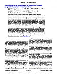
Fig. 1.

The lane detection vision module schema

for high-curvature roads, roundabouts and intersections where extended road models should be applied. The layout for the lane detection system is shown in Fig 1. The raw image from the camera is processed as RGB and grayscale image before being used by three image cues: Canny edge filter-Hough transform cue, LoG edge filter cue and Colour segmentation cue. A particle filter handles the hypotheses about the vehicle state and passes these particles to the cues for testing. Each cue tests all of the particles and assigns a probability to each. The final belief is then formed by the particle filter based on total evaluation from each separate cue. III. PARTICLE F ILTERING Particle filtering is also known as Condensation or Monte Carlo algorithm and is based on Bayesian probabilistic reasoning under Markov assumption (past and future data are independent if the current state of the system is known)[7],[9],[10]. If the previous belief about the state of the system is Bel(xt−1 ), the action model is P (xt |xt−1 , at−1 ) representing the transition from previous state xt−1 , the sensor model is P (ot |xt ) representing the observations at the current instant t and ηt is the normalization factor, then the recursive Bayesian formula for the final belief Bel(xt ) at the current instant t can be described as: Z Bel(xt ) = ηt P (ot |xt ) P (xt |xt−1 , at−1 )Bel(xt−1 )dxt−1 (1) Representing the continuous probability density function (pdf) by a set of n weighted samples also called particles is computationaly more efficient and proves satisfactory also for representation of multi-modal non-Gaussian belief states if the number n is sufficiently large: n o (i) (i) Bel(xt ) ≈ xt , ωt (2) i=1,2,...,n

(i) xt

where is a sample state of the random variable xt , called (i) a pose and ωt an importancy weight factor representing probability measure of each particle. In the case of straightline model of the road, a possible position of the n ego-vehicle is o (i) (i) (i) (i) a sample in the state space defined as xt = Lt , dt , ϕt (i)

with the probability ωt

associated to this hypothesis.

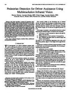
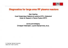
Fig. 2.

The particle filter cycle

The particle filter cycle at each time step comprises of four parts as is shown in Fig 2. Firstly, a group of particles that received best probability estimates from the previous step are resampled from the whole particle set, a fraction of particles are resampled around the best belief particle to refine the search in that region and a certain number of particles are resampled in the whole state space (uniformly random). The later enables resolving the relocalization problem where the particle filter may lost track due to disturbances such as obstacles in the image or brightness intensity change where i.e. standard Kalman filtering may fail. Secondly, particles are diffused according to the error model of the action sensors (in the automotive case these are typically the translational and rotational velocity of the vehicle). Thirdly, the action model takes into account the motion of the system where for the automotive case this is generally the Ackermann motion model [11]. Finaly, when particles are diffused in the state space they each represent a hypothesis that has to be tested against the current vision information from the cues. For an i-th (i) (j) (i) particle xt the j-th cue gives a probability P (ot |xt ) (j) where the observation ot depends on the particular image representation of each cue. Total discrete a-posteriori pdf for the sensor model of the whole state space xt is given as: P (ot |xt ) =

m Y

(j)

P (ot |xt )

(3)

j=1

Combining probabilities from different cues using product operation implies that no cue should return probability 0 since then information would be lost from other cues. Therefore, each cue may return only a probability between [α, 1] with α being the lowest probability measure that may also vary depending on the general performance of each cue (typically set to α = 0.1). In general, the combining and normalization step may be performed also by using a weighted sum of contributions of each cue. However, by using product of probability measures to infere the total probability the preferred combinations are those where each single contribution is approximately equally likely. This can be seen when comparing normalized probability cubes of two random variables X1 , X2 for summation and product case in Fig 3 and Fig 4.

Fig. 3. Probability cube for summation based inference

Fig. 4. Probability cube for product based inference

In the summation based inference, the extremal case of the value of one variable being very likely and the other variable being very unlikely may get an equal total probability as in case when they are both equally likely. In the product based inference the extremal cases are more suppressed. Thus, for a liable result all cues must give a sufficiently high confidence. This feature is expoited furthermore in testing of each single cue where the probabilities of detected position for the left and right lane boundary must be high for both boundaries resulting in a more stable and robust inference scheme. The lowest probability measure in cue testing is denoted as po (typical value 0.01). IV. C UE T ESTING To test each particle a number of cues can been developed. Each cue measures how well the image information matches what would be expected if the particle correctly described the current state of the vehicle. It uses this to assign a probability as to the likeliness that the particle is correct. This section describes the three image cues that have currently been implemented. A. Canny Edge - Hough Transform Cue Canny edge detector processes gray-scale image in multiple stages [12]. The image is first smoothed by a Gaussian convolution mask and then a 2-D first derivative operator is applied to highlight the regions of high contrast - edges in the image. Edges give rise to ridges of high gradient magnitude, however these ridges may be wide and broken, therefore an adaptive threshold nonmaximum supression is performed by a recursive edge neighbourg search to extract accurately the position of a single pixel based connected edge. Such edges are suitable for line detection algorithms [13]. A typical highway scene image is shown in Fig 5.

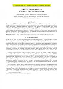
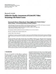
Fig. 5.

A Canny filter edge image with the winning particle (red lines)

For small curvature roads the long straight line segments may represent the road boundaries, lane markings or other objects, smaller size line segments may represent dashed lane markings or other. However, trying to apply a neighbourhood based line detection algorithm directly in the image space may not be suitable for two major reasons. Firstly, the length of the line segments in the image is not known in advance. For instance, dashed lane markings that actually represent the same road boundary will result in different line segments in the image that may be difficult to segment in a postprocessing step. Secondly, in a real road scene road boundaries may be occluded by other objects, in particular by other vehicles, which render neighbourhood based line algorithms difficult to use. Moreover, trying to overlay a perspective road mask in the image space is not liable since single pixel edges of the Canny filter do not provide enough hits for the mask summation. In order to detect line segments, the Hough transform [13] is used in this work since it is invariant to pixel position in an image. This implies that it is not neccessary to distinguish between full or dashed lane markings, marked road edges or natural road boundaries as long as the intensity difference is sufficient for the Canny filter response. Essentialy, it transforms edge pixels in image space that lie along the same straight line to a single point in Hough space. The coordinates of this point are the distance ρ of the line to an origin and the angle θ the line makes to the Ox-coordinate axis. Its implementation requires a two dimensional accumulator array where each cell corresponds to a small span of line parameters ρ and θ. Ordinarily, every possible line going through each edge element is plotted in Hough space as a sine curve. An actual line detected in a particular accumulation cell is then the overlap of all these curves rendering the processing slow. However, by using the angle direction information of the first derivative operator each edge pixel can be transformed directly to a unique accumulator cell by increasing only the total count I of that cell which significantly speeds up the processing time. The Hough transform image of the Canny edge map in Fig 5 is shown in Fig 6 where darker points represent accumulator cells with a higher intensity value I. It is visible that the lane boundaries where the ego-vehicle is placed occupy very confined regions of the accumulator array, i.e. the center of the left lane boundary lying at coordinates (θ, ρ) = (59◦ , 105) and the right lane boundary center lying at (−51◦ , 78) (transformation origin in the upper left corner). To derive a probability measure of each particle according to the straight-line model, the left and right edges of the hypothesized lane n o are converted n to two oHough point centers (i) (i) (i) (i) (i) (i) cl = θcl , ρcl and cr = θcr , ρcr , respectively. Fig 7 shows left (blue colour) and right (green colur) lane positions for each particle of the particle set. Several particles might have one same edge point in Hough space but differ in other. Since both lane boundaries may differ significantly in intensity and structure, the particle edges must be tested and normalized separately. For instance, alignement of a particle’s

Fig. 6.

Hough transform image

pixels with same gradient direction error margin in the image space have a different spread in the ρ component depending on the choice of transformation origin and the pixel position in the image whereas the θ component spread depends only on the gradient direction error itself. For instance, if the upper left corner of the image is chosen as the transformation origin the pixels most sensitive to this error belong to the right lane edge. Since the edge’s cluster has a larger spread (see Figure 6) the measure of alignement to the circular treshold region is less accurate resulting also in less accurate right lane boundary detection. Therefore, to increase robustness of the estimated lane position two Hough transforms are used for each particle. (i) (i) The probability evaluations become ωL and ωR where L and R denote the transformation origin at the upper left and right image corner, respectively. These origins are chosen as to minimize the ρ error sensitivity at values of θ at 45◦ . The nominal angle in real road scene is around 55◦ for the left lane edge to the L origin and right lane edge to the R origin. Attempting to use a single centrally placed transformation origin is also not robust enough and transforms points to all 4 angle quadrants (as opposed to 3 that are needed here). The final probability measure then becomes: (i)

Fig. 7. Left and right lane positions of the particle set (blue and green colour respectively)

(i)

hypothesized left edge center cl to the left lane boundary cluster of N points with intensity values I (k) in Hough space that are found q within the circular treshold region with radius 2 2 rtresh = (θtresh ) + (ρtresh ) is best when the particle’s edge is placed in the center of the real road cluster. The probability measure describing this is: q 2 2 (i) (i) N X (rtresh − (θcl − θ(k) ) + (ρcl − ρ(k) ) ) (k) (i) δcl = I rtresh k=1 (4) The treshold values θtresh and ρtresh are determined such that if the road lane is bounded by a lane marking which generally transforms in two distinguished edges, both edge peaks are included as a single road bondary cluster (i.e. lane marking is taken to occupy 8% of the standard road width). This can be distinctly seen in Fig 6 for the left lane boundary (the cluster radius is enlarged for clarity). The total probability ωCanny (i) of a particle for the cue is determined by taking both left and right edge boundaries into account: (i)

(i)

ω (i) Canny = ωL ωR

(6)

B. Laplacian of Gaussian Edge Cue The LoG filter performs a Laplacian 2nd-order spacial derivative of a Gaussian smoothed grayscale image. A zerocrossing detection of the gradient magnitude image enables extraction of edges which in general may be thicker than single pixel based edges of the Canny edge detector. Thus, this type of edges is suitable for comparison with a perspective model mask that is overlaid directly in image space. The mask is taken to be left and right stripes that are lane marking size wide, determining a generic non-lane region which may also be the road boundary with no lane markings. Fig 8 depicts a LoG edge map which is overlaid by the winning particle’s perspective model mask (yellow). The stripes height is limited to exclude the far-sight region close to the vanishing point where other vehicles may represent false lane boundary detection.

(i)

δcl − δclmin δcr − δcr min + po )( + po ) δclmax − δclmin δcr max − δcr min (5) Using a first derivative operator, in this case the Sobel operator, to determine the gradient direction inherently involves an error [13]. This reflects upon the Hough transformation where

ωCanny (i) = (

Fig. 8. A LoG filer edge image with the perspective model mask of the winning particle

The edge map can be regarded as a binary map, i.e. I (k) =

{0, 1} where every edge pixel represents a positive hit. Each particle generates a different perspective model mask where a simple measure of edge pixel count within the total mask pixel count Nl,r of the left l and right r stripe represents the probability measure for each side of the lane: Nl,r (i) δl,r

=

X

(k)

Il,r

(7)

k=1

The probability measure of the i-th particle is then: (i)

(i)

δl − δlmin δr − δr min + po )( + po ) (8) δlmax − δlmin δr max − δr min The zero-crossing detection phase involves searching for pixel neighbourhood where the 2-nd-order derivative of the image changes sign. By using a larger neighbourhood mask and appropriate smoothing noise variance the edges can be further enhanced, i.e. thickened for a more robust comparison to the perspective model mask. ωLoG (i) = (

C. Colour Cue Colour cue performs comparison of the RGB input image to the mean values R, G, B of each component of the road surface colour. If a pixel’s RGB values lie within the treshold defined by all three variances σR , σG , σB it is considered to be of the road colour. Thus, a binary delta map can be acquired which is used for particle testing. The perspective mask that is overlaid on the delta map in this case includes both left and right lane boundaries which must be of non-road colour and the central region which must be of road colour (Fig 9).

Fig. 9. A delta colour image with the perspective model mask of the winning particle

V. R ESULTS The lane-tracking module has been tested using a single SONY DFW-VL500 camera mounted inside of a Smart Car. The camera is connected to a Pentium IV laptop through a firewire hub. Currently the motion sensors of the vehicle are not integrated in the system therefore only image processing was used to extract the lane position without any motion model. The module was tested in several typical real-road conditions that are shown in Fig 10 through Fig 21. The lane detection module proved robust under different road conditions. If a cue performs poorly at a certain instant the contribution of other cues to the probabilistic measure diminishes its negative effect to the overall performance. This is particulary the case with the Colour cue which is quite sensitive to brightness change and shadow areas on the road. A multimodal colour histogram distribution instead of a single mean for each colour component may improve its performance. In general, the Canny edge filter in combination with Hough transform proved to be the most robust cue that responds immediately to a change in scene since it retains information both about edge magnitude and direction, adapts to different levels of noise and is pixel position insensitive. LoG filter is isotropic and does not contain the edge direction information, thus it may become less stable when other obstacles occlude the lane boundary view, in changing lanes situations or on roads with large shadow areas. Moreover, the LoG and Colour cue are tested directly in the image space on pixel masks which increases significantly the processing time in comparison to small edge pixel number of the Canny cue. The case of dirty front window showed potential to tackle worse visibility conditions particulary due the adaptive Canny filter which is also suitable for abrupt lightning changes such as small tunnels, however, this assumption was not extensively tested. The system detected correctly the near-sight contours of the lane even for higher curvature roads which may be sufficient information for an i.e. lane keeping module. However, using the straight-line model does not allow to place correctly the objects in the far-sight view in the overall environment representation. VI. C ONCLUSION

A vision module was presented for lane detection in vehicles that forms the basis of a driver assistance navigation Similar to the LoG filter, for each part of the perspective module. Edge detection and colour image filters were used (i) mask a δl,r,c measure is calculated representing pixel hit of to extract information about the road environment of the ego non-road or road colour within the total mask area and the vehicle. The information was processed within a probabilistic final probability measure of the i-th particle is: framework using particle filtering where the belief about the state of the system was described by a discrete set of particles (i) (i) each representing a possible solution within the state space. δl − δlmin δr − δr min (i) ωColour = ( + po )( + po ) Particles were assigned a probabilistic measure according to δlmax − δlmin δr max − δr min evaluation against image filters called cues and the particle (i) δc − δcmin ( + po ) (9) with the best total probability measure from all cues described δcmax − δcmin the most likely position of the vehicle. At each instant a new R, G, B and σR , σG , σB are calThe single camera experimental setup mounted in a vehicle culated based on the winning particle information, rendering was tested in various real-road conditions, such as highway the cue adaptive to lightning condition changes. traffic scenes and lane changing, magistral road in inner town

Fig. 10.

Highway - heavy traffic

Fig. 11. Highway - high curvature

Fig. 12. Highway - a front car occluding the view

Fig. 13. Highway - changing lanes (1)

Fig. 14. Highway - changing lanes (2)

Fig. 15. Magistral road - inner city

Fig. 16. Magistral road - ambigous lane border position

Fig. 17. signs

Fig. 18. lane

Fig. 19. Magistral road - leaving a small tunnel

Fig. 20. vature

Magistral road - country

with different ground signs and magistral road in outer city areas with different lightning conditions, road shadows and windscreen visibility. The vision system performed robustly in most cases except in situations where road edges were too obscured by dark areas in outer city areas and in ambiguous positions on the border between two lanes where flickering between two lanes may have occured since no vehicle dynamics was included due to lack of vehicle motion sensors. In comparison with the LoG edge cue and Colour segmentation cue that are based on particle testing in image space, the Canny edge filter with double Hough transform particle testing performed significantly better in terms of robustness and computation speed. This cue presents a good basis for developement of a higher curvature road model from the straight-line road model that is currently being used. ACKNOWLEDGMENT This project was partially funded by the European Commission Contract No. IST-507859 (http://www.sparc-eu.net/). R EFERENCES [1] A.M. Lützeler, E.D. Dickmanns, ”Road recognition with MarVEye”, Proceedings of the IEEE Intelligent Vehicles Symposium 98, Stuttgart, Germany, October 1998, pp. 341-346. [2] T.M. Jochem, D.A. Pomerleau, C.E. Thorpe, ”MANIAC: A next generation neurally based autonomous road follower”, Proceedings of the Third International Conference on Intelligent Autonomous Systems, Pittsburg, PA, February 1993.

Magistral road - high cur-

Magistral road - ground

Fig. 21. Magistral road - dirty windscreen

[3] A. Broggi, M. Bertozzi, A. Fascioli, G. Conte, Automatic Vehicle Guidance, ”The Experience of the ARGO Vehicle”, World Scientific, Singapore, 1999. [4] Massimo Bertozzi, Alberto Broggi, Alessandra Fascioli, Vision-based intelligent vehicles: State of the art and perspectives, Robotics and Autonomous Systems 32 1 - 16, 2000. [5] J.D. Crisman, C.E. Thorpe, ”UNSCARF, a color vision system for the detection of unstructured roads”, Proceedings of the IEEE International Conference on Robotics and Automation, Sacramento, CA, April 1991, pp. 4962501. [6] L. Michael Beuvais, C. Kreucher, ”Building world model for mobile platforms using heterogeneous sensors fusion and temporal analysis”, Proceedings of the IEEE International Conference on Intelligent Transportation Systems 97, Boston, MA, November 1997, p. 101. [7] Nicholas Apostoloff and Alexander Zelinsky, ”Vision In and Out of Vehicles: Integrated Driver and Road Scene Monitoring”, Proceedings of the International Symposium of Experimental Robotics (ISER2002), Italy, 2002. [8] Xu Youchun, Wang Rongben, Libling, Ji Shouwen, A vision navigation algorithm based on liner lane model, Proceedings of the IEEE Intelligent Vehicles Symposium, Dearborn (MI), USA, 2000. [9] Sebastian Thrun, Dieter Fox, Wolfram Burgard, and Frank Dellaert, Robust monte carlo localization for mobile robots, Artificial Intelligence Journal, 2001. [10] Michael Isard and Andrew Blake, Condensation-conditional density propagation for visual tracking, Int. J. Computer Vision, 1998. [11] Uwe Kiencke, Lars Nielsen Automotive control systems, Springer, Inc. 2000. [12] J. Canny, A computational approach to edge detection, IEEE Trans. Pattern Analysis and Machine Intelligence, 1986, vol.8, pp 679-698. [13] Robert M. Haralick, Linda G. Shapiro Computer and Robot Vision Vol.1, Addison-Wesley Publishing Company, Inc. 1992.