hep-lat/9509079 25 Sep 1995. DESY 95{178. HLRZ 95{58. HUB-EP{95/15. September 1995. A Lattice Evaluation of the Deep-Inelastic Structure. Functions of ...
DESY 95{178 HLRZ 95{58 HUB-EP{95/15 September 1995
A Lattice Evaluation of the Deep-Inelastic Structure Functions of the Nucleon� M. Gockeler1 2, R. Horsley3, E.-M. Ilgenfritz3, H. Oelrich1, H. Perlt4, P. Rakow5 , G. Schierholz6 1 and A. Schiller4 ;
;
hep-lat/9509079 25 Sep 1995
1
Hochstleistungsrechenzentrum HLRZ, c/o Forschungszentrum Julich, D-52425 Julich, Germany 2 Institut f ur Theoretische Physik, RWTH Aachen, D-52056 Aachen, Germany 3 Institut f ur Physik, Humboldt-Universitat, D-10115 Berlin, Germany 4 Fakultat f ur Physik und Geowissenschaften, Universitat Leipzig, D-04109 Leipzig, Germany 5 Institut f ur Theoretische Physik, Freie Universitat, D-14195 Berlin, Germany 6 Deutsches Elektronen-Synchrotron DESY, D-22603 Hamburg, Germany Abstract
The lower moments of the unpolarized and polarized deep-inelastic structure functions of the nucleon are calculated on the lattice. The calculation is done with Wilson fermions and for three values of the hopping parameter �, so that we can perform the extrapolation to the chiral limit. Particular emphasis is put on the renormalization of lattice operators. The renormalization constants, which lead us from lattice to continuum operators, are computed perturbatively to one loop order as well as non-perturbatively. Talk given by G. Schierholz at the Workshop QCD on Massively Parallel Computers, Yamagata, March 1995 �
1
1 Introduction For our theoretical understanding of the short-distance structure of the nucleon, as well as for a successful explanation of the recent HERA and polarized lepton-nucleon scattering data, a calculation of the deep-inelastic nucleon structure functions from rst principles is needed. The theoretical basis for such a calculation is the operator product expansion. The quantities of primary interest are the lower moments of the quark and gluon distribution functions and their higher-twist counterparts. We have initiated a program to compute the moments of the unpolarized, F1 and F2, and polarized nucleon structure functions, g1 and g2 , on the lattice. First results of our calculation have been reported in Ref. [1]. In this talk we shall focus on two topics: the valence quark distribution and the spin content of the nucleon. The calculation of the gluon distribution functions and the distribution functions involving sea quarks is in progress. Because of space limitations we shall not be able to discuss the higher moments of g1 and the structure function g2 . Thus we shall concentrate on the moments hxn 1i, where x is the fraction of the nucleon momentum that is carried by the quarks, and �q, the quark spin contribution to the nucleon spin. We have where
hxn 1i(f ) = vn(f );
(1)
1 Xh~p;~sjO(f ) j~p;~si = 2v(f )[p � � � p �n traces]; n �1 f�1����n g 2 ~s � i �n 1 $ ( f ) (2) D �2 � � � D �n q traces O�1 ����n = 2 q� �1 $ with q = u(d) for f = u(d). Here f� � �g means symmetrization of the indices. Furthermore we have �q = 21 a(0f ); (3) where
h~p;~sjO�5(f )j~p;~si = a(0f )s� ; O�5(f ) = q� � 5q: (4) The lattice calculation is performed on a 163 � 32 lattice at gauge coupling �
6=g2 = 6:0. We work in the quenched approximation where one neglects the e�ect of virtual quark loops. We use Wilson fermions, and we compute simultaneously at three values of the hopping parameter, � = 0:155; 0:153 and 0:1515, so that we can extrapolate our results to the chiral limit. This translates into physical quark masses 2
mq of roughly 70, 130 and 190 MeV, respectively. So far we have collected of the order 1000, 600 and 400 independent con gurations at the three � values. The lattice operators O are obtained from the operators in the euclidean continuum, up to factors of i, by replacing the covariant derivative in (2) by the lattice covariant derivative ! D �(x; y) = 12 [U�(x)�y;x+^� U�y (x �^)�y;x �^]: (5) We rst compute the two- and three-point correlation functions X C (t; ~p) = ;� hB� (t; ~p)B� (0; p~)i; �;
X
C (t; �; p~; O) =
�;
� (0; p~)i: ;� hB� (t; ~p)O(� )B
(6)
As our basic proton operator we use (with C = 4 2 in our representation)
B�(t; ~p) =
X
~x;a;b;c
e
ip~~x
�abcua�(x)(ub(x)C 5dc (x)):
(7)
The nucleon matrix elements of interest are then obtained from the ratio
R(t; �; p~; ; O) = C (t; �;~p; O)=C 1 (1+ 4)(t; ~p) 2
E~p 1 Tr [ N J N ] = 21� E + ~p mN 4 (for 0 � � � t), where N = (E~p 4 ip~~ + mN )=E~p and J is de ned by
h~p;~sjOj~p;~si = u�(~p;~s)J u(~p;~s):
(8) (9)
In order to increase the overlap with the ground state and to make the plateau region { by this we mean the region where the excited states have died out { in � as broad as possible, we use `Jacobi smearing' [2]. We smear both source and sink. In Fig. 1 we show the e�ective nucleon mass for � = 0:155, i.e. our lightest quark mass, as given by ln(C (t)=C (t + 1)). We nd a good plateau. Our results for the hadron masses are compiled in Table 1. The chiral limit is obtained by extrapolating in 1=� to m� = 0. If we assume that m2� vanishes linearly with 1=� ! 1=�c , we obtain the critical value �c = 0:15693(4).
3
m� m� mN
0.1515 0.504(2) 0.570(2) 0.900(5)
� 0.153 0.422(2) 0.507(2) 0.798(5)
0.155 0.297(2) 0.422(2) 0.658(5)
Table 1: The hadron masses in lattice units at = 6:0.
eff
m
N
t
Figure 1: E�ective nucleon mass plot. Both source and sink are smeared. The horizontal line indicates the result of the t as well as the t interval. 4
Observable hxi hx2i hx3i �q
hOi v2 v3 v4 a0
Components
O BO Of44g 31 (Of11g + Of22g + Of33g) 163 -1.892(6) 25 -19.572(10) Of114g 21 (Of224g + Of334g) 3 Of1144g + Of2233g Of1133g Of2244g 157 15 -37.16(30) 5 O2 0 15.795(3)
Table 2: The lattice operators. The momentum is taken to be ~p = (2�=16; 0; 0) � (p1; 0; 0) in the case of v3 and v4 and ~p = 0 elsewhere. In our calculation of the three-point functions we have xed t at 13. For the unpolarized case we have taken = 12 (1 + 4). For the polarized case we have chosen = 12 (1 + 4)i 5 2, which corresponds to polarization + - in the 2-direction. For the calculation of the higher moments we need non-vanishing nucleon momenta. We have taken ~p = 0 and ~p = (2�=16; 0; 0) � (p1; 0; 0).
2 Renormalization of Lattice Operators
The bare lattice operators, O(a), which are in general divergent, must be renormalized appropriately before we can use them. We de ne nite operators O(�), renormalized at the scale �, by O(�) = ZO ((a�)2; g(a))O(a); (10) where we de ne (11) hq(p)jO(�)jq(p)i = hq(p)jO(a)jq(p)i jtree p2 =�2 ; jq(p)i being a quark state of momentum p. In the limit a ! 0 this de nition amounts to the continuum, momentum subtraction renormalization scheme. The numbers that we will quote later on will all refer to this scheme. The lattice operators must be constructed such that they belong to a de nite irreducible representation of the hypercubic group H (4) [3, 4]. In particular they must not mix with lower-dimensional operators. In this talk we will consider the operators listed in Table 2. We have computed the renormalization constants of these operators (and others) in perturbation theory to one loop order [1, 5]. (See also Ref. [6].) We write 2 ZO ((a�)2; g) = 1 16g�2 CF [ O ln(a�) + BO ];
5
(12)
Z
µ2
Figure 2: The non-perturbatively determined renormalization constant Zv2 as a function of �2. The solid line represents the perturbative result given in Table 2. Z
µ2
Figure 3: The non-perturbatively determined renormalization constant Za0 as a function of �2. The solid line represents the perturbative result given in Table 2. The dashed line is the result of tadpole improved perturbation theory. 6
where CF = 4=3 and O is the anomalous dimension that also enters the Wilson coe�cients. The results of our calculation are listed in Table 2. In case of v3 there is a small mixing problem [5], which we have ignored here, because numerically it is insigni cant. The e�ect of renormalization can be relatively large, in particular for those operators that involve higher powers of covariant derivatives. The main sources of contribution are the leg and operator tadpole diagrams. There has been a lot of discussion in the literature [7] on how to reorganize perturbation theory around these contributions in order to achieve a better convergence of the perturbative series. It is important to determine the renormalization constants accurately. In view of this we have computed the renormalization constants non-perturbatively as well [8], following the suggestion of Ref. [9]. The renormalization constants are obtained from the calculation of the operator matrix element (13) hq(p)jO(a)jq(p)i jp2=�2 : For this calculation we need to x the gauge. We have chosen the Landau gauge, and we average over all Gribov copies. In Figs. 2 and 3 we show our results for Zv2 and Za0 as a function of �2 (in lattice units). Here � = 0:153, but we do not see any dependence on �. We compare the non-perturbative results with the perturbative calculation. (The renormalization scheme used in the non-perturbative calculation di�ers slightly from the perturbative one. But the di�erence is insigni cant [8].) We nd remarkably good agreement between the two approaches. In Fig. 3 we have also shown the prediction of tadpole improved perturbation theory [7]. The non-perturbative result lies in between the perturbative and the tadpole improved result, so nothing seems to be gained by tadpole resummation in this case. But we will have to wait until we have computed all renormalization constants non-perturbatively before we can draw any rm conclusions. In the following we shall take �2 = a 2 � 2GeV2; (14) which eliminates the logarithms in the renormalization constants, and we will denote ZO (1; g = 1:0) by ZO .
3 A Selection of Results We are now ready to compute the nucleon matrix elements (2) and (4). The physical matrix elements at the scale � are obtained from the ratios (8) by Rv2 = Z1 21� mN v2; Rv3 = Z1 21� p21v3; v2 v3 (15) 1 1 i 1 m N 2 Rv4 = Z 2� Ep1 p1v4; Ra0 = Z 2� 2E a0: v4 a0 p1 7
u
d
1/κ
u
d
1/κ
u
d
1/κ
Figure 4: The moments hxn 1i as a function of 1=�, together with a linear t to the data. The solid circles indicate the extrapolation to the chiral limit. The diamonds mark the phenomenological valence quark distribution of Ref. [10] ( t D ). 8
∆q u
d
1/κ
Figure 5: The quark spin contribution to the proton spin as a function of 1=�, together with a linear t to the data. The solid circles indicate the extrapolation to the chiral limit. We have made sure that we are computing the matrix elements of the lowest-lying state, i.e. the nucleon. We nd that the signal is practically constant for distances of � larger than two lattice spacings from the source p (t = 0) and from the sink (t = 13). We have de ned the continuum quark elds by 2� times the lattice quark elds. For the renormalization constants we take the perturbative values given in Table 2. The results are plotted in Figs. 4 and 5. All our results are given for the proton. The distribution functions of the neutron are obtained by interchanging u and d. The rst observation we make is that the nucleon matrix elements show roughly a linear behavior in 1=� � 1=�c + 1:8mq a; (16) i.e. in the quark mass. The lines drawn in Figs. 4 and 5 are linear ts to the data. The result of the extrapolation is indicated by the solid circles. Let us next discuss the moments hxn 1i. We nd that the lowest moment is practically independent of the quark mass, while for growing n the dependence on the quark mass increases. As the lower moments of the distribution functions are dominated by the small-x region, this means that at small x quark mass e�ects are negligible. At intermediate and large x, on the other hand, the distribution functions depend strongly on the magnitude of the quark mass. In the limit of large quark masses the moments approach the predictions of the non-relativistic quark model. In particular we nd hxn 1 i(u) � 2hxn 1 i(d) for all n. In Fig. 4 we have compared our results with the phenomenological valence quark distribution functions [10]. For the lowest moment the lattice result turns out to be 9
signi cantly larger than the phenomenological value, while for the largest moment we nd the opposite situation. This holds for both, u and d quark distributions. Thus the lattice calculation predicts a valence quark distribution that is larger at intermediate to small x and smaller at large x than the phenomenological distribution function. At present we have no explanation for this discrepancy. Let us now discuss �q. Sea quark e�ects may be neglected for heavy quarks, and they drop out in the di�erence �u �d. In the chiral limit we obtain �u �d � gA = 1:07(9):
(17)
This is to be compared with the experimental value of the axial vector coupling constant gA = 1:26. A recent lattice calculation of the sea quark contribution [12] nds ��u = �d� = 0:14(5), ��s = 0:13(4), where we have used the perturbative renormalization factor. If we add these numbers to our results, we obtain for the total quark spin contribution to the nucleon spin �� = 0:18(8):
(18)
This is in agreement with the result of a full QCD calculation [13] which includes dynamical quark loops.
4 Conclusion We have presented some results of a high statistics calculation of the lower moments of the polarized and unpolarized deep-inelastic structure functions of the nucleon. The calculation has been performed in the quenched approximation, and it was done for three di�erent quark masses. This allowed us to extrapolate our results to the chiral limit. The lattice data are rather accurate now, so that it is equally important to determine the renormalization constants precisely. We have computed the renormalization constants in perturbation theory to one loop order as well as non-perturbatively. So far we nd consistent results. The valence quark distributions that we have obtained on the lattice di�er from the phenomenological distribution functions. This was also observed before [14]. One explanation could be that at smaller values of Q2 higher twist contributions are nonnegligible, which have not been included in the phenomenological analysis. We plan to investigate this possibility in the future. Our results for �q are consistent with experiment. It is interesting to see how the results vary with the quark mass. At large quark masses our results agree largely with what one would expect on the basis of the quark model. For small quark masses there are, however, signi cant changes. 10
Acknowledgments This work was supported in part by the Deutsche Forschungsgemeinschaft. G. S. likes to thank A. Nakamura for his kind hospitality.
References [1] M. Gockeler, R. Horsley, E.-M. Ilgenfritz, H. Perlt, P. Rakow, G. Schierholz and A. Schiller, Nucl. Phys. B (Proc. Suppl.) 42 (1995) 337; DESY preprint DESY 95-128 (1995) (hep-lat/9508004). [2] C. R. Allton et al., Phys. Rev. D47 (1993) 5128. [3] M. Baake, B. Gemunden and R. Oedingen, J. Math. Phys. 23 (1982) 944, ibid. 23 (1982) 2595 (E). [4] J. Mandula, G. Zweig and J. Govaerts, Nucl. Phys. B228 (1983) 109. [5] M. Gockeler, R. Horsley, E.-M. Ilgenfritz, H. Perlt, P. Rakow, G. Schierholz and A. Schiller, in preparation. [6] G. Martinelli and Y. C. Zhang, Phys. Lett. B123 (1983) 433; S. Capitani and G. Rossi, Nucl. Phys. B433 (1995) 351; G. Beccarini, M. Bianchi, S. Capitani and G. Rossi, Rome preprint ROM2F/95/10 (1995) (hep-lat/9506021). [7] G. P. Lepage and P. B. Mackenzie, Phys. Rev. D48 (1993) 2250. [8] M. Gockeler, R. Horsley, E.-M. Ilgenfritz, H. Oelrich, H. Perlt, P. Rakow, G. Schierholz and A. Schiller, in preparation. [9] G. Martinelli, C. Pittori, C.T. Sachrajda, M. Testa and A. Vladikas, Nucl. Phys. B445 (1995) 81. [10] A. D. Martin, W. J. Stirling and R. G. Roberts, Phys. Rev. D47 (1993) 867. [11] J. Ellis and M. Karliner, Phys. Lett. B341 (1995) 397. [12] M. Fukugita, Y. Kuramashi, M. Okawa and A. Ukawa, KEK Preprint 94-173 (1994); S. J. Dong, J.-F. Lagae and K.-F. Liu, Kentucky Preprint UK/95-01 (1995). [13] R. Altmeyer, M. Gockeler, R. Horsley, E. Laermann and G. Schierholz, Phys. Rev. D49 (1994) R3087. [14] G. Martinelli and C. T. Sachrajda, Nucl. Phys. B316 (1989) 355; G. Martinelli, Nucl. Phys. B (Proc. Suppl.) 9 (1989) 134. 11