robot team should be decomposed into a sequence of sub-goals and ... ation scheme for robot soccer where the environment is represented in different time ... nal results of the games played during a limited time period for predicting the ... goalkeeper for determining the optimal scoring policy in RoboCup 2D Simula-.
A Layered Metric Definition and Evaluation Framework for Multi-robot Systems C ¸ etin Meri¸cli and H. Levent Akın Department of Computer Engineering Bo˘ gazi¸ci University ´Istanbul, TURKEY {cetin.mericli,akin}@boun.edu.tr
Abstract. For succesful accomplishment the top-level goal of a multirobot team should be decomposed into a sequence of sub-goals and proper sequences of actions for achieving these subgoals should be selected and refined through execution. Selecting the proper actions at any given time requires the ability to evaluate the current state of the environment, which can be achieved by using metrics that give quantitative information about the environment. Defining appropriate metrics is already a challenging problem; however, it is even harder to assess the performance of individual metrics. This work proposes a layered evaluation scheme for robot soccer where the environment is represented in different time resolutions at each layer. A set of metrics defined on these layers together with a novel metric validation method for assessing the performance of the defined metrics are proposed.
1
INTRODUCTION
In a multi-robot system, both individual robots and the entire team are confronted with a set of decisions for achieving both short-term and long term goals. In order to make a decision, one needs to evaluate the current situation of the environment. Evaluation of the current situation requires statistically consistent quantitative metrics but both defining appropriate metrics and validating them are challenging processes. Robot soccer is a good platform to test and develop multi-agent applications because it has some physical limitations such as limited and noisy sensorial information and limited moving capability as in the real life and it also has a highly dynamic, real-time environment. Definition of metrics for performance evaluation of multi-robot systems is is not a deeply investigated research topic so far. VerDuin et al. drew the attention on the importance of evaluating the performance evaluation metrics by investigating the efficiencies of different criteria used in model evaluation in machine learning [1]. Yavnai proposed a set of metrics for classification of system
autonomy [2]. Horst applied previously published Naive Intelligence Metric on autonomous driving problem [3]. Olsen and Goodrich proposed six metrics for evaluating human computer interactions [4]. Balch has proposed a metric called Social Entropy based on Shannon’s Information Entropy for measuring the behavioral diversity of a team of homogeneous robots [5]. On evaluating real soccer games, Rue and Salvesen applied Markov Chain Monte Carlo method on the final results of the games played during a limited time period for predicting the possible results of the forthcoming games [6]. Yanco discussed the methods of defining metrics for robot competitions in order to be able to judge the participants efficiently [7]. In the RoboCup domain, Kok et al. used the distance and the orientation of the ball with respect to the opponent goal, and the position of the opponent goalkeeper for determining the optimal scoring policy in RoboCup 2D Simulation environment [8]. Dylla et al. have initiated a qualitative soccer formalism for robot soccer [9]. They proposed a top-down approach to the soccer knowledge, following the classical soccer theory. Quantitative information like the distance and orientation to the ball, distance and orientation to the opponent goal and distance to the nearest teammate are widely used in role assignment or individual behavior selection [10, 11]. Quinlan et al. proposed to use more high-level measurements like the goal difference and the remaining time to the end of the game in determining team aggression level [12]. In this work, we propose a three-layered decomposition of a soccer game in which each layer deals with the system at a different time resolution. A set of metrics built on top of position information of players and the ball in three different time resolutions are also presented. Finally, a novel, contingency table based validation method for metric consistency is given. The main contributions of this work are: – Metric validation problem is stated as a challenging problem where autonomous decision making systems are in use. – A novel statistical method is proposed for addressing the metric validation problem. – A three-layered decomposition of the soccer game is given and a set of metrics are defined on different time resolutions. Organization of the rest of the paper as follows: In Section 2, proposed approach is explained in detail. Section 3 contains explanation of metric validation process and finally, we conclude and point out some future works in Section 4.
2
PROPOSED APPROACH
The most primitive information we can estimate in the environment is the position information of players and the ball so we defined a set of metrics calculated from the position information for different time resolutions. It is assumed that the positions of opponent players are also known with a degree of error.
Since there are both team-level long-term goals and individual-level shortterm goals, we need a game decomposition in different time resolutions. We propose three layers defined on different time resolutions in a game: – Instantaneous Level – Play Level – Game Level 2.1
Instantaneous Metrics
Instantaneous metrics are calculated from one time-step position information. Since getting the control of the ball is the most important sub-task, most of the metrics are proposed for evaluating the chance of getting control of the ball. Convex Hull Metrics Convex Hull of a set of points is defined as the smallest convex polygon in which all of the points in the set lies. In an analogous manner, by substituting points with the players in the soccer, we obtain a new concept: Convex Hull of a Team. We propose two metrics involving the convex hull of a team: – The Area of Convex Hull tends to measure the degree of spread of the team over the field. The value of this metric increases as the team members are scattered across the field. – Density of Convex Hull is applied only if the ball falls within the convex hull. The formal definition of the density is given in Equation 1. PN p Density =
i=1
(Xplayer(i) − Xball )2 + (Yplayer(i) − Yball )2 N
(1)
where, N is the number of players on the corners of the convex hull. If the ball is in the own half of the field, the goalkeeper is included in the convex hull calculation. If the ball is in the opponent field, the goalkeeper is excluded. The density value is calculated only if the ball falls within the convex hull. If the ball falls outside of the convex hull, then the value of the metric is 0. The probability of the ball falling within the convex hull increases as the area of convex hull increases and it is expected that if the ball falls within the convex hull, the probability of getting the control of the ball increases. On the other hand, it is expected that the probability of getting the control of the ball increases as the density of the convex hull increases. Vicinity Occupancy Vicinity Occupancy measures the ratio of the teams players to the opponent players within a vicinity of the object of interest. The formal definition of the vicinity occupancy is given in Equation 2. Occupancy =
Pown − Popp Pown + Popp
(2)
Fig. 1. Convex Hulls of two teams at a time point
where, Pown is the number of own players in the vicinity of the object of interest, Popp is the number of opponent players in the vicinity, and P is the total number of players in the vicinity. The result is a real number in the interval [−1, 1] where −1 means that the vicinity is dominated by the opponent players, 0 means that there is no dominance and finally, 1 means that the vicinity is dominated by our players. Vicinity Occupancy is calculated for three objects of interest: – Ball – Own Goal Area – Opponent Goal Area The ball is the most important object in the game. Dominating the vicinity of the ball can be interpreted as having the control of the ball since the probability of controlling the ball increases as the number of own players in the vicinity increases and decreases as the number of opponents in the vicinity increases.
Fig. 2. a) Occupancy in the vicinity of Ball. b) Occupancy in the vicinity of Own Goal
Dominating the vicinity of own goal is desired since it can be interpreted as a good defensive tactic. Dominating the vicinity of opponent goal is basically
the opposite situation of occupancy of own goal case. As a result, in the ideal case, it is desired to dominate vicinities of both ball and goals but dominating the ball vicinity is the most important issue. Pairwise separation Metrics Pairwise separation is aimed to measure the degree of separation of an object of interest with opponent team. Equation for calculation of pairwise separation is given in Equation 3. Pn Pn Pm i j k i=1 j=1 k=1 separates(Pown , Pown , Popp , Object) SObject = 2 (3) ( 1 if Line(P1 , P2 ) intersects Line(P3 , Object), separates(P1 , P2 , P3 , Object) = 0 otherwise. (4) where, n is the number of own players, m is the number of opponent players, and Pown and Popp are the sets of own and opponent players, respectively.
Fig. 3. Pairwise separation of Ball from Opponent Team: Robots pointed with light arrows are separated from the ball
Pairwise separation depends on the assumption that if an opponent player is separated from the object of interest, it is more likely for us to prevent it from accessing the object of interest. For example, if the pairwise separation value for ball is high, our chance to control the ball will also be high. Since separation test is performed for each player and with each teammate, each tuple is counted twice. So, the calculated separation value is divided by 2 to eliminate this double count. Clearance of the path between two points Clearance metric measures the accessibility of one point from another point. Clearance depends on the existence and positions of players and their movement capability. It is assumed that a player has control over an area called Area of
Impact. The size and shape of area of impact depends on locomotional abilities of the robot. For a robot with omnidirectional movement and shooting ability with any side (for example Teambots robots or MIROSOT robots), shape of the area of impact will be a circle. The area of impact depends on the speed of the robot. A fast robot would have a larger area of impact than a slower robot. The area of impact of a robot is considered as a physical obstacle along with the body of the robot when calculating the clearance. If the path between two points is occluded by the area of impact of at least one opponent player, it is considered that the way between the two points is not clear. We calculate three clearance metrics: – Clearance to the ball – Clearance of ball to the opponent goal – Clearance of ball to the teammates Once a player reaches to the ball, there are three actions it can take: – Shooting to the goal – Dribbling with the ball – Passing the ball to a teammate Since it is assumed that the player must reach the ball before shooting or passing, only the clearance of the ball to the opponent goal and to the teammates are important. Sample clearance situations are shown in Figure 4.
Fig. 4. a) Clearance to the Ball. b) Clearance to the Opponent Goal for the Ball. c) Clearance of the Ball to the Teammates
2.2
Play Level Metrics
Play level metrics tend to measure the two important issues in the soccer game: Reachability of a position from another position and ball possession. The proposed predicates isReachable(P ositionf rom , P ositionto ) and hasBall( Player )
are calculated by using instantaneous metrics over a time period. Both isReachable and hasBall are boolean metrics so we need to map the output of the metric combination from a real number to a boolean value. isReachable Predicate The function isReachable(P ositionf rom , P ositionto ) returns True if the path between points P ositionf rom and P ositionto is clear from obstacles (Sec. 2.1). Since clearance metrics are instantaneous metrics and can be quite noisy, clearance is calculated by examining the consecutive values of the clearance metrics. If the path between two positions is Clear for consecutive N time-steps, isReachable is set to True. Contrarily, if the path between two positions is Occluded for consecutive N time-steps, isReachable is set to False. Determining the number N is another optimization problem. Since such an optimization is beyond the scope of this work, we arbitrarily select N = 10 and leave finding the optimal value of N as a future work. hasBall Predicate hasBall is used to check whether a certain player has the ball possession or not. hasBall(P layer) returns True if the Player has the ball possession or not. As in the isReachable predicate, output is calculated from the values of the metrics developed for measuring the ball possession over a number of consecutive time-steps. We used the same value of 10 for the window size variable N for calculating the value of the hasBall. 2.3
Game Level Metrics
Game level metrics are proposed for measuring the statistics about the game over a long time period. All game level metrics try to measure the dominance of the game. Three metrics are calculated in game level: – Attack/Defense Ratio – Ball Possession – Score Difference Attack/Defense Ratio Attack/Defense Ratio (ADR) tends to measure the dominance of the game by comparing the longest time the ball spends in our possession area in the game field with the longest time the ball spends in opponent possession area. Possession areas are defined as goal-centered semi-circles. The radius of the circle is a hyper-parameter and it needs some machine-learning and optimization techniques for finding the optimal value of the radius, but we simply select the radius of the circle as half of the field height. The Attack/Defense Ratio is the difference of largest consecutive time-steps that the ball is in opponent possession area and the largest consecutive number of time-steps that the ball is in our own possession area divided by the sum of them. Formula for Attack/Defense Ratio is given in Equation 5. ADR =
P osown − P osopp P osown + P osopp
(5)
This value is a real number in the interval [−1, 1]. A positive value of this metric indicates that the ball is spending more time in the opponent possession field than it spends in own possession field meaning that our team is more aggressive and dominating the game. Ball Possession Ball Possession (BP) measures the dominance of the game by comparing the longest time our team has the ball possession with the longest time opponent team has the ball possession. Play Level predicate hasBall is used in the calculation of ball possession. Formula for Ball Possession is given in Equation 6. BP =
Ballown − Ballopp Ballown + Ballopp
(6)
where Ballown is the number of consecutive time steps that hasBall(P layerown ) is True for one of our players. Ballopp is the number of consecutive time steps that hasBall(P layeropp ) is True for one of the opponent players. A positive value of the metric indicates that our team has the control of the ball more than the opponent team. Score Difference Score difference (SD) is probably the most popular and trivial metric which is calculated from the scores of the teams. The equation for calculating score difference is given in Equation 7. SD = Scoreown − Scoreopp
(7)
The result is an integer indicating the dominion over game so far.
3
EVALUATING METRICS
For the evaluation of defined metrics, a total of 200 games were played with our team against four different opponents in Teambots simulation environment [13]. In order to reveal the performance of the opponent teams in all aspects and to eliminate ceiling and floor effects in evaluating the performance of our own team, we have tried to use stratification in selecting the opponent teams so we choose both weak, moderate and powerful teams as opponents. After the games are played and the position data for the players and the ball are recorded, each game is divided into episodes which starts with a kick-off and ends with either a score or end of half or end of game whistle. Episodes ending with own scores are marked as positive examples and episodes ending with opponent scores are marked as negative examples. Episodes ending with end of half or end of game whistle are ignored. At the end of 200 games, 81 negative and 1016 positive episodes were recorded. Each episode is then divided into smaller sequences of time-steps that are separated by a touch (or kick) to the ball. These sub-episodes are also marked as positive/negative examples
depending on which team has touched the ball at the end of the sub-episode. If the ball is kicked by own team and the previous kick was performed by the opponent team, that sub-episode is marked as a Positive example. If the ball is kicked by opponent players and the previous kick was made by home players, that sub-episode is marked as a Negative example. The sub-episodes that are started and ended with the kicks of same team are ignored. Then, the marked sub-episodes are used to evaluate metrics related to the ball possession. 3.1
Metric Validation
Proposing metrics is a challenging task but it is even harder to evaluate the performance of a metric. We use metrics to obtain quantitative information about the environment but how can we be sure that the metric we proposed really measures the property it is supposed to measure. So we are confronted with another challenging problem: Metric validation. In order to consider a metric as informative, the metric should show the same trends in the same situations. For example, we can propose the distance to the ball metric for assessing the probability of getting the control of the ball. However, distance might not be the right indicator. So we should check whether the distance metric has the same trends in positions having the same ending (our team got the control of the ball, or opponent team got the control of the ball). Due to noise and sudden changes in positions of ball and other players, recorded metric data contain noise making the observation of trends in metric data difficult. In order to extract trends in recorded noisy data, some smoothing algorithms are applied to the recorded data. We have tried two smoothing algorithms on the recorded metrics: – 4253h,Twice Smoothing – Hodrick-Prescott Filter 3.2
4253h, Twice Smoothing
In 4253h, Twice algorithm, running median smoothers with window sizes 4, 2, 5 and 3 are applied consecutively. Then Hanning operator is applied. Hanning operator replaces each data point Pi with Pi−1 + P2i + Pi+1 4 4 . Then the entire operation is repeated [14]. Performing two or three consecutive 4253h, Twice resulted in great reduce in noise but the trend extraction is still hard in resultant smoothed data. 3.3
Hodrick-Prescott Filter
Hodrick-Prescott filter is proposed for extracting underlying trend in macroeconomic time series [15]. In the Hodrick-Prescott (HP) Filter approach, the observable time series yt is decomposed as: yt = gt + ct
(8)
where gt is a non-stationary time trend and ct is a stationary residual. Both gt and ct are unobservable. We think yt as a noisy signal for the gt . Hence, the problem is to extract gt from yt . HP Filter solves the following optimization problem: M in T {gt }t=1
T X t=1
2
(yt − gt ) + λ
T X
[(gt+1 − gt ) − (gt − gt−1 )]2
(9)
t=2
where λ is a weight for a signal against a linear time trend. λ = 0 means that there is no noise and yt = gt . As λ gets larger, more weight is allocated for the linear trend. So as λ → ∞, gt approaches to the least squares estimate of yt ’s linear time trend. Selecting the value of λ is another design problem. In our work, we used 14400 as the value of the λ which is used to smooth monthly data in original implementation.
Fig. 5. Smoothing: a) Raw data, b) 4253h,Twice, c) Hodrick-Prescott Filter
Figure 6.a shows the kicks in which the team with the ball possession is changed. In Figure 6, bold spikes denotes the kicks that are performed by our team and preceding by an opponent kick and, narrow spikes denotes the kicks that are performed by the opponent team and preceding by an own kick. In order to test the correlation among the sub-episodes with the same mark (positive or negative), a straight line is fitted on metric data in the sub-episode by using Least Squares Fitting. Then, the possible correlation between the mark of the sub-episode and the sign of the first derivative of the fitted line (i.e. slope of the line) is investigated. It is expected that the signs of the slopes of fitted lines on the metric data in sub-episodes with the same mark are the same. In Figure 6.b, fitted lines on the pairwise separation of the ball metric data between two kicks can be seen. It is seen in the figure that the fitted lines to the positive sub-episodes have positive slopes where the fitted lines to the negative sub-episodes have negative slopes. Table 1 shows that the pairwise separation of the ball metric has a positive correlation with the sub-episode mark. Whenever the metric shows an increasing
Fig. 6. a) an example Pairwise Separation of the Ball Metric with positive and negative kicks. b) after fitting a Least-Squares Line to the metric Table 1. The Kick-Slope distribution for Pairwise Separation of the Ball
Positive Trend Negative Trend
Own Kick Opponent Kick 94 27 19 50
trend, our own team performs a kick and since performing a kick requires the ball possession, it can be said that if the pairwise separation of the ball metric shows an increasing trend, our own team has the ball possession. Nearly all of the metrics have some hyper-parameters that we chose arbitrarily in this work. With arbitrarily selected hyper-parameters, only the pairwiseseparation metrics have shown consistent behaviors. Exploring the consistency of the metrics with different values of hyper-parameters is left as a future work.
4
CONCLUSIONS
In this work, we have proposed a decomposition of soccer game into layers dealing with different time resolutions, a set of metrics and a validation method for testing the consistency (hence, the informativeness) of a metric. Some of the metrics are novel and a metric validation method is proposed for the first time. Although the proposed decomposition is applied on robot soccer, it is not limited to soccer and can be adapted to any multi-robot system. Some of the major contributions of this work can be listed as: – Stating the metric validation problem as a challenging problem where autonomous decision making systems are in use. – Proposing a novel statistical method for addressing the metric validation problem.
– Proposing a three-layered decomposition of the soccer game and a set of metrics on these layers at different time resolutions. Nearly all of the metrics have some hyper-parameters so there is a large room for conducting machine learning based research on finding optimal values of these hyper-parameters. Finding such hyper-parameters, developing methods for dealing with uncertainty in real life, investigating the possibility of a spatial decomposition of the soccer and combining metrics defined on different layers of both spatial and temporal decompositions are left as future work.
5
ACKNOWLEDGMENTS
This work is supported by TUBITAK Project 106E172.
References 1. William.H.VerDuin, Ranganath Kothamasu, and Samuel.H.Huang. Analysis of performance evaluation metrics to combat the model selection problem. In PERMISA Workshop, 2003. 2. Arie Yavnai. An information-based approach for system autonomy metrics part i: Metrics definition. In PERMISA Workshop, 2003. 3. John A. Horst. Exercising a native intelligence metric on an autonomous on-road driving system. In PERMISA Workshop, 2003. 4. Dan R. Olsen and Michael A. Goodrich. Metrics for evaluating human-robot interactions. In PERMISA Workshop, 2003. 5. T. Balch. Social entropy: a new metric for learning multi-robot teams. In 10th International FLAIRS Conference (FLAIRS-97), 1997. 6. H˚ avard Rue and Øyvind Salvesen. Predicting and retrospective analysis of soccer matches in a league. 7. Holly A. Yanco. Designing metrics for comparing the performance of robotic systems in robot competitions. In Workshop on Measuring Performance and Intelligence of Intelligent Systems (PERMIS), 2001. 8. Jelle Kok, Remco de Boer, and Nikos Vlassis. Towards an optimal scoring policy for simulated soccer agents. Technical report, 2001. 9. F. Dylla, A. Ferrein, G. Lakemeyer, J. Murray, O. Obst, T. Rfer, F. Stolzenburg, U. Visser, and T. Wagner. Towards a league-independent qualitative soccer theory for robocup. In 8th International Workshop on RoboCup 2004 (Robot World Cup Soccer Games and Conferences, 2004. 10. M. Veloso, S. Lenser, D. Vail, M. Roth, A. Stroupe, and S. Chernova. Cmpack-02: Cmu’s legged robot soccer team. Technical report, 2002. 11. Thomas R¨ ofer et. al. Germanteam 2006. Technical report, The GermanTeam, 2007. 12. Michael J. Quinlan, Naomi Henderson, and Richard H. Middleton. The 2006 nubots team report. Technical report, Newcastle Robotics Laboratory, 2007. 13. Tucker Balch. Teambots, 2000. http://www.teambots.org. 14. P. R. Cohen. Empirical Methods for Artificial Intelligence. MIT Press, Massachusetts, 1995. 15. R. J. Hodrick and E. C. Prescott. Postwar u.s. business cycles: An empirical investigation. Journal of Money, Credit and Banking, 29, 1997.