Dec 15, 2011 - tron (MLP), where all weights are modified at each learning step. Furthermore .... Figure 1: Illustration of the cLVQ Learning Rule. Based on a ...
A Life-Long Learning Vector Quantization Approach for Interactive Learning of Multiple Categories Stephan Kirstein1,2 , Heiko Wersing1 , Horst-Michael Gross2 and Edgar K¨orner1 1
Honda Research Institute Europe GmbH Carl-Legien-Str. 30, 63073 Offenbach am Main, Germany 2
Ilmenau University of Technology Neuroinformatics and Cognitive Robotics Lab P.O.B. 100565, 98684 Ilmenau, Germany
Abstract We present a new method capable of learning multiple categories in an interactive and lifelong learning fashion to approach the “stability-plasticity dilemma”. The problem of incremental learning of multiple categories is still largely unsolved. This is especially true for the domain of cognitive robotics, requiring real-time and interactive learning. To achieve the life-long learning ability for a cognitive system, we propose a new learning vector quantization approach combined with a category-specific feature selection method to allow several metrical “views” on the representation space of each individual vector quantization node. These category-specific features are incrementally collected during the learning process, so that a balance between the correction of wrong representations and the stability of acquired knowledge is achieved. We demonstrate our approach for a difficult visual categorization task, where the learning is applied for several complex-shaped objects rotated in depth. 1. Introduction Humans are able to acquire and maintain knowledge during their complete lifetime. This outstanding ability is called life-long learning (Bagnall, 1990). In contrast to this, artificial neural networks are typically only adapted during their learning phase and their weights, representing the learned knowledge, are fixed afterwards. Such a static learning architecture can be powerful in constrained and stationary environmental settings but may not be suitable for technical applications like assistive robots or interactive agents. This is because these systems require a continuous error correction and need to enlarge their knowledge base to operate in changing and unpredictable environments. Our target is to propose a novel categorization approach that enables interactive and life-long learning in high-dimensional sensory feature spaces. This enforces particular requirements on the learning architecture: The assumption of an unpredictably changing learning environment forces the learning system to self-adapt its representation parameters. Scalability to a large number of categories requires efficient memory usage. Learning in direct interaction with humans needs realtime update of the stored category representations. And finally the ability of learning multiple categories at the same time provides a great advantage for an efficient and natural human training dialog with the learning system (the isolated training of single categories induces an explosion of individual category exemplars that must be shown). The fundamental problem of life-long learning with artificial neural networks is the so-called “stability-plasticity dilemma”. Here the term plasticity refers to the ability of a learning system to incorporate new acquired knowledge into its internal representation. Plasticity can be achieved Preprint submitted to Elsevier
December 15, 2011
with incremental neural networks like the growing neural gas (Fritzke, 1995). For this architecture the training process starts with a minimal network size and iteratively increases the network size based on an insertion criterion. The final network dimensionality then reflects the complexity of the current learning task. However, already learned knowledge should also be preserved to guarantee the stability of previously learned information, posing the largely unsolved stability problem. This challenge occurs if a network model is trained with a limited and changing training ensemble for life-long learning tasks, making it infeasible to store all experiences during the complete operation time of the system. Therefore in this paper we are particularly interested in incremental learning of representations under the condition, where a particular training vector can only be accessed for a limited time period. As a consequence the training with such a changing data ensemble typically causes the well-known “catastrophic forgetting effect” (French, 1999): With the incorporation of newly acquired knowledge, the previously learned knowledge is quickly fading out. Closely related to this effect is the term “catastrophic interference” (McCloskey & Cohen, 1989): Patterns of different categories which are similar in feature space, confuse the learning and overwrite earlier presented patterns. The requirements for life-long learning architectures are also dependent on the targeted recognition task. For identification tasks, where the target is the separation of a specific instance (e.g. one particular physical object) from all other instances, the combination of incremental learning with stability considerations of consolidated network parts are typically sufficient (Kirstein et al., 2008). In contrast to this, for categorization tasks the mapping from several object instances to a shared attribute (e.g. the basic shape) is required. This means for the example of visual categorization, where an individual object (e.g. red-white car) typically belongs to several different categories, a decoupled representation for each category (“red”, “white” and “car”) has to be learned. This decoupling provides a more efficient representation and a higher generalization performance compared to object identification architectures. It can be achieved using additional metrical adaptation or feature selection methods. However, due to the fact that exemplars of a category are incrementally presented, considerable changes to the feature weighting and selection can occur. Therefore for categorization tasks a balance between the stability of knowledge and the correction of wrong category representations must be found. This balance complicates the learning of such representations compared to identification tasks. Finally we consider feature weighting and selection methods without a priori assumptions as advantageous for learning of arbitrary categories. To satisfy our requirements for life-long learning we combine an exemplar-based neural network with a category-specific feed-forward feature selection method, where the interactive and life-long learning of both parts is the major novelty of our proposed method. Although our approach is applicable for any kind of categories we concentrate in this paper on a challenging visual categorization task of rotated complex-shaped objects. In the following we discuss related work addressing life-long learning, feature selection, visual categorization and online learning in more detail. 1.1. Life-Long Learning Architectures One of the first attempts to approach the “stability-plasticity dilemma” led to the development of the adaptive resonance theory (ART) and especially Fuzzy ARTMAP (Carpenter et al., 1992). This network architecture is widely accepted but is known to be sensitive to the noise level, to the presentation order of the training data and to the selection of the vigilance parameter (Polikar et al., 2001). This parameter controls the maximal size of the hypercubical receptive field of a single ART node and therefore is crucial with respect to the generalization capability. Furthermore ART is also unsuited for high-dimensional and sparse feature representations (Kirstein et al., 2008) that are required for our visual categorization task. Similarly to the ART network family life-long learning architectures are typically based on exemplar-based learning techniques like learning vector quantization (LVQ) (Kohonen, 1989) or 2
growing neural gas (GNG) (Fritzke, 1995). Such neural architectures are beneficial for life-long learning, because for a specific input vector the learning methods modify only small portions of the overall network. Thus stability can be better achieved compared to the multi-layer perceptron (MLP), where all weights are modified at each learning step. Furthermore the learning of exemplar-based networks is commonly based on some similarity measurements (e.g. Euclidean distance), where the chosen metric has a strong impact on the generalization performance. To relax this dependency, metrical adaptation methods can be used that individually weight the different feature dimensions as proposed for the generalized relevance learning vector quantization (GRLVQ) (Hammer & Villmann, 2002) algorithm. A common strategy for life-long learning architectures is the usage of a node specific learning rate combined with an incremental node insertion rule (Hamker, 2001; Furao & Hasegawa, 2006; Kirstein et al., 2008). This permits plasticity of newly inserted neurons, while the stability of matured neurons is preserved. The major drawback of these architectures is the inefficient separation of co-occurring categories, because typically the complete feature vectors are used to represent the different classes and no assignment of feature vector parts to different classes is considered. Other approaches to the “stability-plasticity dilemma” were proposed by Polikar et al. (2001) and Ozawa et al. (2005). Polikar et al. (2001) proposed the “Learn++” approach that is based on the boosting (Schapire, 1990) technique. This method combines several weak classifiers to a so-called strong classifier based on a majority-voting schema, where the weak classifiers are incrementally added to the network and afterwards are kept fixed. The proposed “Learn++” can therefore be used for life-long learning tasks, but for more complex learning problems a large amount of such weak classifiers are required to represent the categories. This makes the method unsuitable for our desired interactive learning capability. In contrast to this Ozawa et al. (2005) proposed to store representative input-output pairs into a long-term memory for stabilizing an incremental learning radial basis function (RBF) network. Additionally it also accounts for a feature selection mechanism based on incremental principal component analysis, but no classspecific feature selection is applied to efficiently separate co-occurring categories. 1.2. Feature Selection Methods In the context of text categorization feature selection methods are a common technique to enhance the performance (Yang & Pedersen, 1997), while for visual categorization tasks feature selection gained distinctly less interest. One exception are approaches based on boosting (Viola & Jones, 2001), where this is an integrated part of the learning method. Category-specific feature selection is considered to be an important part for our categorization approach. Commonly only a small subset of extracted features is relevant for a specific category, while the other features are irrelevant or even can cause confusions. Furthermore small category-specific feature subsets are beneficial with respect to the computational costs to allow fast interactive learning. Therefore in the following a brief overview of different feature selection techniques is given. There are basically three groups of feature selection methods, namely filter, wrapper and embedded methods (Guyon & Elissee, 2003). Filter methods (see Forman (2003) for an overview) are independent from the used classifier and commonly select a subset of features as a pre-processing step. The corresponding feature selection is typically based on some feature ranking method (Furey et al., 2000; Kira & Rendell, 1992), but also the training of single variable classifiers is used. The second group of feature selection methods are wrapper methods (Kohavi & John, 1997). Similar to the filter approaches these wrapper methods are independent from the underlying recognition architecture but they use the learning algorithm as a “black box” to weight different feature subsets (e.g. based on the training error). Due to the incorporation of the learning method to guide the feature selection process and to evaluate the different feature subsets, wrapper methods are considered to select better sets compared to filter methods (Guyon & Elissee, 2003). Wrapper methods 3
furthermore can be categorized into backward and forward selection methods, where the backward selection starts with a full set of features and iteratively eliminates irrelevant features. In contrast to this, forward selection methods start with an empty set of features and incrementally add new features. The major advantage of the backward selection methods is that they can detect combination features very efficiently. This enables good performance even for less class-specific feature sets. Although forward selection methods require distinctly more class-specific single features they are faster and thus preferable for interactive learning tasks. The last group of feature selection methods are the so called embedded methods. Here the feature selection is an integrated part of the recognition architecture and is typically optimized together with the network parameters, so that these methods usually can not be transferred to other learning approaches. One strategy of this group is to add sparsity constraints to the error function (Perkins et al., 2003), which prune out irrelevant network connections. 1.3. Visual Category Learning Approaches In the recent years many architectures dealing with categorization tasks have been proposed in the computer vision research field. Such category learning approaches can be partitioned into generative and discriminative models (Fritz, 2008). Generative probabilistic models, as proposed by Leibe et al. (2004), Fei-Fei et al. (2003), Fergus et al. (2003) or Mikolajczyk et al. (2006), first model the underlying joint probability P (x, tc ) for each category tc and all training examples x individually and afterwards use the Bayes theorem to calculate the posterior class probability p(tc |x) (Bishop, 2006). The advantages of generative models are that expert knowledge can be incorporated as prior information and that those models usually require only a few training examples to reach a good categorization performance. In contrast to this, discriminant models directly learn the mapping from x to tc based on a decision function Φ(x) or estimate the posterior class probability P (tc |x) in a single step (Ng & Jordan, 2001). Common approaches for this group of categorization models are based on support vector machines (Heisele et al., 2001), boosting (Viola & Jones, 2001; Opelt et al., 2004) or SNOW (Agarwal et al., 2004). Such discriminant models tend to achieve a better categorization performance compared to generative models if a large ensemble of training examples is available (Ng & Jordan, 2001). In general most of these categorization approaches are robust against partial occlusions, scale changes, and are able to deal with cluttered scenes. However, many models have only been demonstrated to work with data sets restricted to canonical views of categories. Thomas et al. (2006) try to overcome this limitation by training several pose-specific implicit shape models (ISM) (Leibe et al., 2004) for each category. After the training of these ISMs, detected parts from neighboring pose-dependent ISMs are associated by so-called “activation links”. These links then allow the detection of categories from many viewpoints. Additionally categorization architectures are commonly designed for offline usage only, where the required training time is not important. This makes them unsuitable for our desired interactive training. Recent work of Fritz et al. (2007) and Fei-Fei et al. (2007) addresses this issue by proposing incremental clustering methods, which in general allow interactive category learning, but still these approaches are restricted to the canonical views of the categories. 1.4. Online and Interactive Learning The development of online and interactive learning systems has become increasingly popular in the recent years (Roth et al., 2006; Steels & Kaplan, 2001; Arsenio, 2004; Wersing et al., 2007). Most of these methods were not applied to categorization tasks, because their learning methods are unsuitable for a more abstract and variable category representation. The work of Skoˇcaj et al. (2007) is of particular interest with respect to online and interactive learning of categories. It enables learning of several simple color and shape categories by selecting a single feature that describes 4
the particular category most consistently. Finally the corresponding category is then represented by the mean and variance of this selected feature (Skoˇcaj et al., 2007) or more recently by an incremental kernel density estimation using mixtures of Gaussians (Skoˇcaj et al., 2008). Although this architecture shares some common targets with our proposed learning method, the restriction to a single feature only allows the representation of categories with little appearance changes. This is basically because more complex categories typically require several features to adequately represent all category instances. To avoid this limitation we propose a forward feature selection process that incrementally selects an arbitrary number of features if they are required for the representation of a particular category. The manuscript is structured as follows: in Section 2 we introduce our category learning architecture that enables interactive and life-long learning of arbitrary categories. Afterwards we describe the feature extraction methods used to extract shape and color features in Section 3. In Section 4 we show the application of our proposed learning method to a visual categorization task. Finally we discuss the results and related work in Section 5 and give the pseudocode notation of our category learning method in Section A. 2. Incremental and Life-Long Learning of Categories Our memory architecture is based on an exemplar-based incremental learning network combined with a forward feature selection method to allow life-long learning of arbitrary categories. Both parts are optimized together to find a balance between insertion of features and allocation of representation nodes, while using as little resources as possible. This is crucial for interactive learning with respect to the required computational costs. In the following we refer to this architecture as category learning vector quantization (cLVQ). To achieve the interactive and incremental learning capability the exemplar-based network part of the cLVQ method is used to approach the ”stability-plasticity dilemma” of life-long learning problems. Commonly for LVQ networks the number of nodes for each class has to be predefined. Thus experiments normally are repeated with different numbers of nodes to find a network size adequate for the difficulty of the corresponding learning problem. Such a repetition of experiments is unsuitable for interactive learning. Thus we define a node insertion rule that automatically determines the number of required nodes. The final number of allocated nodes corresponds to the difficulty of the different categories itself, but also to the within-category variance. Finally the long-term stability of these incrementally learned representation nodes is considered as proposed by Kirstein et al. (2008). Additionally for our learning approach a category-specific forward feature selection method is used to enable the separation of co-occurring categories, because it defines category-specific metrical “views” on the nodes of the exemplar-based network. During the learning process it selects lowdimensional subsets of category-specific features by predominantly choosing features that occur almost exclusively for a certain category. Furthermore only these selected category-specific features are used to decide whether a particular category is present or not. This enables computational efficiency and interactive learning, which especially for high-dimensional data is typically difficult to achieve. For guiding this selection process a feature scoring value hcf is calculated for each category c and feature f . This scoring value is only based on previously seen exemplars of a certain category, which can strongly change if further information is encountered. Therefore a continuous update of the hcf values is required to follow this change. 2.1. Distance Computation and Learning Rule The learning in the cLVQ architecture is based on a set of high-dimensional and sparse feature vectors xi = (xi1 , . . . , xiF ), where F denotes the total number of features. We define the changing 5
Positive representative
Category 1
Category 2
Low−dimensional subspace
Low−dimensional subspace
Negative representative Training vector xi Decision Boundary
k (2)
w min
... ...
...
i
Label vector t : i i i i tC−1 tC t1 t 2 +1 −1 0 −1
w
...
Training vector xi
kmin(1)
kmin(C)
w
Category C−1
Category C
Low−dimensional subspace
Low−dimensional subspace
cLVQ Nodes wK
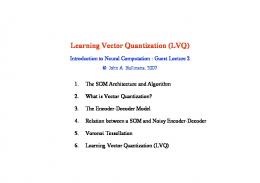
Figure 1: Illustration of the cLVQ Learning Rule. Based on a training vector xi and the corresponding target vector ti the winning nodes wkmin (c) are calculated for each category c independently. For this calculation only the selected features f ∈ Sc are used, so that the categorization decision is based on the different low-dimensional feature subsets. If the categorization decision was correct the winning node wkmin (c) is shifted into the direction of the training vector. Otherwise wkmin (c) is moved in the opposite direction. If for an xi the membership of a category is unknown (tic = 0) no adaptation of the prototype node wkmin (c) is performed.
training set T as a subset of all available vector indices i. Additionally each vector xi is assigned to a list of category labels ti = {ti1 , . . . , tiC }. We use C to denote the current number of represented categories, where each tic ∈ {−1, 0, +1} labels an xi as positive or negative example of category c. The third state tc = 0 is interpreted as unknown category membership, which means that all vectors xi with tic = 0 have no influence on the representation of category c. The cLVQ representative vectors wk with k = 1, . . . , K are built up incrementally, where K denotes the current number of allocated vectors w. Each wk is attached to a label vector uk , where ukc ∈ {−1, 0, +1} is the model target output for category c, representing positive, negative, and missing label output, respectively. Each cLVQ node wk can therefore represent several categories c. For the category-specific distance computation dc we use a weighted Euclidean distance with specific weight factors λcf related to the generalized relevance learning vector quantization (GRLVQ) method proposed by Hammer & Villmann (2002): dc (xi , wk ) =
F X
λcf (xif − wfk )2 ,
(1)
f =1
where the category-specific weights λcf are updated continuously. We denote the set of selected features for an active category c ∈ C as Sc . We choose λcf = 0 for all f 6∈ Sc , and otherwise adjust it according to a scoring procedure explained later. The winning nodes wkmin (c) (xi ) are calculated independently for each category c. Let Ac = {k|ukc 6= 0} be the set of indices of representatives that represent category c. If Ac = ∅, since no representative is yet available for this category, or
6
tic = 0 no weight adaptation is done. Otherwise we compute: kmin (c) = arg min dc (xi , wk ). k∈Ac
(2)
Each wkmin (c) (xi ) is updated based on the standard LVQ learning rule (Kohonen, 1989), but is restricted to feature dimensions f ∈ Sc : k
wf min
(c)
k
:= wf min
(c)
k
(c)
+ µ Θkmin (c) (xif − wf min ) ∀f ∈ Sc ,
(3)
where µ = 1 if the categorization decision for xi was correct, otherwise µ = −1 and the winning node wkmin (c) will be shifted away from xi . This node adaptation is illustrated in Fig. 1. Additionally Θkmin (c) is the node-dependent learning rate as proposed by Kirstein et al. (2008): Θ
kmin (c)
akmin (c) . = Θ0 exp − γ !
(4)
Here Θ0 is a predefined initial value, γ is a fixed scaling factor, and ak is an iteration-dependent age factor. The age factor ak is incremented every time when the corresponding wk becomes the winning node. 2.2. Feature Scoring and Category Initialization The incremental category learning of our model is organized in training epochs, where only a limited number of category entries (e.g. object views) are visible to the learning method, emulating a limited short-term memory (STM). After each epoch some of the training vectors xi and their corresponding target category values ti are removed and replaced by vectors of a new instance to test the life-long learning capability of the cLVQ method. Therefore for each training epoch the scoring values hcf , used for guiding the feature selection process, are updated in the following way: hcf =
Hcf ¯ cf . Hcf + H
(5)
¯ cf are the number of previously seen positive and negative training examples The variables Hcf and H of category c, where the corresponding feature f was active (xf > 0). For each newly inserted object view, each counter value Hcf is updated in the following way: Hcf := Hcf + 1 if xif > 0 and tic = +1,
(6)
¯ cf is updated as follows: and H ¯ cf := H ¯ cf + 1 if xif > 0 and tic = −1. H
(7)
The score hcf defines the metrical weighting in the cLVQ representation space. We then choose λcf = hcf for all f ∈ Sc and λcf = 0 otherwise. Finally if category c with the category label tic = +1 occurred for the first time in the current training epoch, we initialize this category c with a single feature and one cLVQ node. We select the feature vc = arg maxf (hcf ) with the largest scoring value and initialize Sc = {vc }. Among all training vectors the one xi ∈ T is selected as the initial cLVQ node, where the selected feature vc has the highest activation, i.e. wK+1 = xq with xqvc ≥ xivc for all i. The attached label vector is chosen as uK+1 = +1 and zero for all other categories. c
7
all errors solved for category c − stop learning
errors for category c occured − start learning
until errors solved or no features left select and add new feature gain > gain ǫmin . else
(13)
For the cLVQ architecture this gradual decrement of insertion thresholds has two benefits. At the beginning of a learning epoch many allocated object-specific network resources are rejected, so that a compact representation is guaranteed. Additionally the ǫmin is selected in a way to also allow the representation of categories for which no category-specific features are available. In such rare cases the categorization performance to new category members is most probably poor, but at least already known exemplars of such a category can be robustly detected. Furthermore all features that were first below the insertion threshold ǫ1 are retested, if meanwhile ǫ1 is below the previously measured performance increase. 3. Feature Extraction We investigate the learning capabilities of our method based on a visual categorization task. Three feature extraction methods are used to provide shape and color information as illustrated in Fig. 4. Although features from different visual modalities are extracted this qualitative separation of the extracted features is not given to the learning system as a priori information. For our categorization task we are particularly interested in discovering the structure of the categories from the high-dimensional but sparse feature vectors by using a flexible metrical adaptation. Assume you want to learn the category “fire engine”, where all training examples are mainly of red color. If the learning of this category is restricted to shape features only, it would be difficult to distinguish 10
blue
Color Histogram
Parts−Based Features Input Image
green red
Feature Vector
0.3
yellow yes blue no duck yes cup unknown
1 −1 1 0
Categories
ti
...
...
Holistic C2 Features
0.8 0.2 0.0 0.0
0.0 0.0 0.5 0.0
xi
0.4
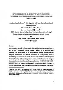
Figure 4: Feature extraction. Color features are extracted as histogram bins in the RGB space. Shape features are obtained from parts-based feature detectors and a feed-forward feature extraction hierarchy. Shape and color features are concatenated into a single “flat” vector representation. The target categories are represented in a category vector ti for each feature vector xi .
the category “fire engine” from other cars and trucks. This is because the most distinctive feature, the red color, is not included in the feature representation. Therefore we let the learning algorithm decide which feature combinations are most suitable to represent a category. As a consequence we concatenate all extracted features of an object view into a single high-dimensional and structureless feature vector xi . Despite the fact that the overall dimensionality is high, typically only a subset of 15-30% of features are activated for any given input , i.e. xif > 0 with 1 ≤ f ≤ F . 3.1. Histogram Binning for Color Feature Extraction For the representation of color information we use the common histogram binning method that combines robustness against view and scale changes with computational efficiency (Swain & Ballard, 1991). Overall Fco = 6x6x6 = 216 histogram bins within the RGB color space are used, where typically a small amount of features are specific for a complete color category. 3.2. Hierarchical Feed-Forward Shape Feature Extraction We use a feed-forward feature extraction architecture inspired by the human ventral visual pathway (Wersing & K¨orner, 2003) as one method to extract shape features. This architecture is based on weight-sharing and a succession of feature detection and pooling stages. The feature detectors are obtained by unsupervised learning based on invariant sparse coding and provide a set of general and less category-specific features. Starting point for the feature extracting process is the input image ji . The first feature-matching layer S1 is composed of four orientation sensitive Gabor filters zm s1 (x, y) with m = 1, . . . , 4, which perform a local orientation estimation. To compute
11
mi the response Pˆs1 (x, y) of a simple cell of this layer, responsive to feature type m at position (x, y) first the input image ji is convolved with a Gabor filter zm s1 (x, y): mi Pˆs1 (x, y) = |ji ∗ zm s1 (x, y)|,
(14)
where the ∗ denotes the inner product of two vectors. Additionally a winners-take-most (WTM) mechanism between features at the same position is performed and a simple threshold function with a common threshold for all cells in layer S1 is applied. We denote the final output of the mi S1 layer at position (x, y) as Ps1 (x, y). The following C1 layer subsamples the S1 output Pmi s1 by pooling down to a quarter in each direction (e.g. 64x64 S1 features are pooled down to 16x16 C1 features): mi Pc1 (x, y) = tanh (Pmi (15) s1 ∗ zc1 (x, y)), where zc1 (x, y) is a normalized Gaussian pooling kernel with width σc1 , identical for all features m, and tanh is the hyperbolic tangent function. The S2 layer is sensitive to local combinations of the orientation estimation features extracted from layer C1. The so-called combination features of this S2 layer (for this experiment 50 different shape features with n = 1, . . . , 50 are used) are trained with invariant sparse coding (see Wersing ni & K¨orner (2003) for details). The response Pˆs2 (x, y) of one S2 cell is calculated in the following way: X ni nm Pˆs2 (x, y) = Pmi (16) c1 ∗ zs2 (x, y), m
znm s2 (x, y)
where is the receptive field vector of the S2 cell of feature n at position (x, y), describing connections to the plane m of the previous C1 cells. Similarly to the S1 layer, a WTM mechanism and a final threshold function are applied in this S2 layer. The final C2 layer again performs a spatial integration and reduces the resolution by half in each direction (i.e. 16x16 S2 features are down-sampled to 8x8 C2 features). For this operation the same pooling mechanism as in layer C1 is used. The final dimensionality of this C2 layer is Fc2 = 50x8x8 = 3200, where the features in one of the 50 feature maps are topographically organized and a single feature responds to a local patch in the original segment ji . 3.3. Parts-based Shape Feature Extraction In contrast to the hierarchical feed-forward feature extraction architecture the parts-based features are trained in a supervised manner with respect to category specificity. We combine these different shape features to show the ability of the category learning method to select appropriate features out of a large number of possible candidates. Such feature combinations are uncommon because most categorization methods exclusively rely on parts-features like in the categorization architectures of Willamowski et al. (2004) or Agarwal et al. (2004). The parts-based feature detection (see Hasler et al. (2007) for details) is based on a preselected set of SIFT-descriptors (Lowe, 2004), which are designed to be invariant with regard to rotations in the image plane. Commonly in categorization frameworks such descriptors are only extracted at a small number of interest points, detected e.g. by the Harris detector (Harris & Stephens, 1988) or the Kadir and Brady detector (Kadir & Brady, 2001). These interest point detectors usually respond to highly textured regions and typically ignore structureless regions. In contrast to this in the present approach these SIFT descriptors are extracted at any location in the segment ji allowing for a greater variety of learnable categories, which also includes visually less structured categories. For each segment ji the similarity Pami (x, y) (m = 1, . . . , 500) between the stored feature detector m ˆ mi (x, y) corresponding to the segment ji at position (x, y) is calculated za and the SIFT-response P a using the dot product: ˆ mi (x, y) ∗ zm Pami (x, y) = P (17) a a 12
i The final response Pami for the feature detector zm a and the current segment j is defined as:
Pami = max(Pami (x, y)).
(18)
x,y
This means that for each feature only the maximum response is used, neglecting all spatial and configurational information. Such information is commonly included in categorization methods like in (Leibe et al., 2004), but requires a high amount of representational resources. Neglecting this information leads to a more compact representation with an efficient reuse and combination of parts, which enhances the learning speed for interactive category learning tasks. As a final step the non-sparse feature activations are transformed into a sparse representation, by choosing for each segment ji only 10% of the features with highest detector responses. 4. Experimental Results In the following section our proposed cLVQ life-long learning architecture is compared with a single layer perceptron (SLP), an incremental support vector machine (SVM) (Martinetz et al., 2009) and two modified cLVQ versions cGRLVQ and cLVQ∗ . The comparison of the exemplarbased networks is done to measure the effect of the proposed feature weighting, and feature selection method with respect to the categorization performance, number of allocated resources and required training time. For this comparison the cLVQ∗ is the most simplified exemplar-based network that is closest to the original LVQ proposed by Kohonen (1989). The only modification is the incremental adding and testing of new prototype nodes, but compared to cLVQ no feature weighting and selection is performed. In contrast to this, the cGRLVQ additionally applies a feature weighting based on the GRLVQ method proposed by Hammer & Villmann (2002). The GRLVQ weighting is based on the distance dcorr to the nearest correctly labeled prototype wkcorr (c) and dincorr to the c c kincorr (c) nearest prototype w with incorrect label: ∆λcf = Θ
λ
Φ′G
dcorr dincorr c c i incorr 2 (x − w ) − (xif − wfcorr )2 , f f incorr corr + dincorr dcorr + d d c c c c !
(19)
where Θλ is the learning rate for the λcf weighting values and Φ′G is the first derivative of a Fermifunction. Similar to the proposed cLVQ this dynamical feature weighting enables the cGRLVQ to suppress irrelevant features but no explicit feature selection is performed. The comparison with the SLP network architecture is done because this is the simplest neural network model that fulfills the requirements of the categorization task. Therefore SLPs are used to measure the baseline performance. For each category one output node is used. The output outslp c of each node is defined as: i outslp c (x ) =
1 , 1 + exp(−wcslp ∗ xi − βc )
(20)
where wcslp is a single linearly separating weight vector with bias βc for each category c. The training is based on standard stochastic gradient descent in the sum of quadratic difference errors between training target and model output. In contrast to the more commonly used receiver operating characteristics (ROC) curves we estimate the rejection thresholds during the learning process, based on the average activation strength of the network output. This is necessary for interactive learning tasks to allow categorization of new object views at any time. Finally our proposed cLVQ method is compared to the established support vector machine (SVM) approach (Cortes & Vapnik, 1995). We expect that the categorization performance of our cLVQ ranges in between the simple SLP and SVM. Nevertheless with the focus on interactive learning the memory consumption and learning speed are as important as the categorization 13
performance. For the SVM comparison we used the SoftDoubleMaxMinOver approach proposed by Martinetz et al. (2009) because of its ability of incremental learning and its computationally efficient learning procedure. Although we use the standard SoftDoubleMaxMinOver approach (Martinetz et al., 2009) for our SVM experiments, we use it in an unusual way. The most common usage of SVMs is that all training and test data is collected a-priori. This has the advantage that the optimal kernel function and parameters can be determined with a grid search and all different parameter sets are evaluated according to their generalization performance. It is obvious that such a grid search is infeasible for fast and interactive learning. Therefore we decided to use linear kernels and a hard margin criterion with C = 106 for all SVM experiments. Nevertheless in a pre-study we also tested RBF kernels, but the simple linear kernels achieved a comparable performance and in contrast to the RBF kernels the results are much less affected by the exact choice of the parametrization. Additionally those linear kernels required much less training time. The selected SoftDoubleMaxMinOver method already supports incremental SVM learning, but so far only increasing sets of feature vectors are considered. In contrast to this we incrementally add new feature vectors at the beginning of each training epoch, while removing the oldest vectors from the training set. Furthermore we reinitialize the SVMs at each training epoch with the current set of support vectors and update them according to the current set of training vectors. Due to the fact that the selected support vectors conserve the most relevant training information from previous learning epochs, we do not expect a strong “catastrophic forgetting effect”. 4.1. Experimental Setup For the comparison of our cLVQ architecture with other learning approaches we use a challenging categorization database composed of views of 56 different training objects and 56 distinct objects for testing (see Fig. 5), which were never used during the training phase. For each object 300 color views of dimensionality 128x128 pixels were taken in front of a black background while rotating the object around the vertical axis. Overall our object ensemble contains ten different shape categories and five different color categories as shown in Fig. 5. It should be mentioned that several objects are multi-colored (e.g. the cans) where not only the base color should be detected, but also all other prominent colors covering at least 30% of the visible object view. This multi-detection constraint complicates the categorization task compared to the case where only the best matching category or the best matching category of a specified group of visual attributes (e.g. one for color and one for shape) must be detected. For all experiments performed with this database we trained the different network architectures with a limited and changing training ensemble T composed of a visible “window” of only three objects to test the life-long learning ability of the different approaches. For each epoch only these three out of all 56 training objects (900 training views) are visible to the learning algorithm. At the beginning of each epoch a randomly selected object is added, while the oldest one is removed. This scheme is repeated until all training objects are presented once to the network architectures. Additionally all experiments are repeated ten times with identical parameter set but random order of object presentation. The corresponding results shown in Fig. 7 and Fig. 8 are the average values over these runs. Furthermore we analyzed our training set with respect to the “catastrophic interference effect”. Therefore the pairwise Euclidean distance of all training vectors, composed of color and partsbased features, are calculated first. Based on this distance matrix we computed for each category a histogram of the intra category similarity. This means that the Euclidean distance of all vector pairs belonging to the same category are considered for such histograms. Additionally we calculated the inter category similarity. Here all training vector pairs are used, where for one view the 14
Training Objects
Test Objects
Rotation Examples
Examples of Multi−Colored Objects
Figure 5: Object Ensemble. Examples of all training (left) and test objects (right) used for our categorization task, where 15 different categories are trained. As color categories red, green, blue, yellow and white are trained. The shape categories are animal, bottle, box, brush, can, car, cup, duck, phone, tool. Each object was presented in front of a black background and is rotated around the vertical axis (bottom), resulting in 300 color images per object.
15
Category Red
Category Blue
Category Green
0.2
0.2
0.2
0.1
0.1
0.1
0
0
2
4
6
8
10
12
14
16
0
18
Category Yellow
0
2
4
6
8
10
12
14
16
18
0
20
Category White
0
0.2
0.2
0.1
0.1
0.1
0
2
4
6
8
10
12
14
16
18
0
20
0
2
4
6
8
10
12
14
16
18
0
20
0
Category Bottle
Category Box 0.2
0.2
0.1
0.1
0.1
0.2
0
0
2
4
6
8
10
12
14
16
18
0
20
0
2
4
6
8
10
12
14
16
18
0
20
8
10
12
14
16
18
20
2
4
6
8
10
12
14
16
18
20
0
2
4
6
8
10
12
14
16
18
20
Category Cup
0.2
0.2
6
Category Brush
Category Car
Category Can
4
Category Animal
0.2
0
2
0.2
0.15 0.1
0.1
0.1
0.05 0
0
2
4
6
8
10
12
14
16
18
Category Duck 0.1
0
2
4
6
0
2
4
6
8
10
12
14
16
18
8
10
12
14
16
18
20
0
20
0.2
0.2
0.1
0.1
0
0
2
4
6
0
2
4
6
8
10
12
14
16
18
20
Category Tool
Category Phone
0.2
0
0
20
8
10
12
14
16
18
20
0
0
2
4
6
8
10
12
14
16
18
20
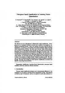
Figure 6: Intra and Inter Category Similarity. Histograms of the pairwise intra (solid lines) and inter category (dashed lines) similarity of all training vectors, based on the Euclidean distance. If both histograms are strongly overlapping, at least for approaches based on the Euclidean distance, the learning of those categories gets more difficult. This overlap is most prominent for the color categories, but also for some of the shape categories the intra and inter category similarity matches strongly.
16
category is present and for the second view the category is not present. The comparison of intra and inter category histograms for a particular category indicates how simple this category can be learned with an Euclidean distance based approach. Typically a stronger match between both histograms complicates the learning of this category. Additionally in such strong overlapping cases the occurrence of the “catastrophic interference effect” becomes more prominent. In Fig 6 it can be seen that especially for the color categories the histograms are almost identical, while for shape categories the overlap is typically smaller. This high inter category similarity of the color categories is most probable due to concatenation of shape and color features, where the amount of different color features in the complete training vector is distinctly less than for the shape features. Additionally our training set is composed of different colored exemplars of a certain shape category, where the larger shape feature portion of those training vectors should be quite similar. This effect can be especially seen in the distinctly higher intra category similarity of most shape categories. 4.2. Setup of Learning Parameters For all LVQ-type neural networks we set the node dependent learning rate Θ0 = 0.000055 and a scaling factor γ = 55 (see Eq. 4). Furthermore for the cGRLVQ and cLVQ∗ 35 iterations are calculated, where during one iteration all training examples are randomly shown once. Both methods incrementally add a single prototypical node after 75 wrongly categorized training vectors. For the cGRLVQ the feature weighting learning rate Θλ was set a magnitude smaller than Θ0 as suggested by Hammer & Villmann (2002). Additionally for a better stability of the cGRLVQ learning process the incremental insertion of nodes was decoupled from the update of the weighting values. In contrast to this for our proposed cLVQ method the allocation of network resources is based on the dynamically calculated feature insertion threshold ǫ1 ∈ [8; 45], node insertion threshold ǫ2 ∈ [15; 100] and α = 0.25 value as explained in Section 2.4. Additionally the maximum number of iterations is set equally to the number of extracted features, but an early stopping is possible if all training errors are resolved. For the SVM experiments the learning rate was set to ΘSV M = 0.000055 and the maximum number of learning steps was set to 257 ∗ 103 , which is the default setting of the used toolbox. For all SVM experiments linear kernels and a hard margin criterion was used. finally for the SLP experiments the learning rate was set to ΘSLP = 0.00055, while the number of iterations was set to 100. A higher number of iterations would strongly reduce the training error, but also increases the “catastrophic forgetting effect” for this kind of neural network. 4.3. Categorization Performance Although no prior information is given during the learning process with respect to the kind of trained categories, we distinguish between color and shape categories in the performance measurement to discuss the different quality of extracted features and the corresponding behavior of all network architectures. We also investigate the effect of different shape features by performing experiments with parts-based features only or the combination of these features with less categoryspecific C2 features. 4.3.1. Color and Parts-based Features The overall performance of the cLVQ architecture for this feature setting is high for all categories as can be seen on the left side of Fig. 7. For the color categories it performs much better than the simpler cGRLVQ and cLVQ∗ . Thus for categories with a few stable and category-specific features a feature selection method and the suppression of irrelevant features is beneficial with respect to the generalization performance. On the contrary for shape categories the cGRLVQ method performs at 17
Color, Parts−based and C2 Features
0.9
0.9
0.85
0.85
Categorization Performance
Color Categories Categorization Performance
Color and Parts−based Features
0.8 0.75 0.7 0.65 0.6 0.55
cLVQ cGRLVQ cLVQ* SLP SVM
0.5 0.45 0.4
0
4
8
12
16
20
24
28
32
36
40
44
48
0.8 0.75 0.7 0.65 0.6 0.55
0.45 0.4
52
cLVQ cGRLVQ cLVQ* SLP
0.5
0
4
8
12
16
20
24
28
32
36
40
44
48
52
Learning Epoch
Learning Epoch
Categorization Performance
Shape Categories Categorization Performance
0.9
0.9 0.8 0.7 0.6 0.5
cLVQ cGRLVQ cLVQ* SLP SVM
0.4 0.3 0.2 0
4
8
12
16
20
24
28
32
36
40
44
48
52
Learning Epoch
0.85 0.8 0.75 0.7 0.65 0.6 0.55
cLVQ cGRLVQ cLVQ* SLP
0.5 0.45 0.4
0
4
8
12
16
20
24
28
32
36
40
44
48
52
Learning Epoch
Figure 7: Comparison of Categorization Performance. For this comparison of our proposed cLVQ with cGRLVQ, cLVQ∗ , SVM, and SLP we performed ten different runs with identical parameter set but random object order. The categorization performance is calculated after each training epoch, based on all test vectors. This means that the performance is calculated based on the representation of the objects seen so far, simulating an interactive learning session. Additionally different feature sets are used to investigate their impact on the categorization performance. In general cLVQ and SVM are superior for color categories compared to all other learning methods, while for the shape categories cLVQ is slightly worse than cGRLVQ and cLVQ∗ and distinctly worse than SVM. Although SVM reaches the highest performance for the combination of color and parts-based features it catastrophically scales with the addition of high-dimensional and less category-specific C2 features. This means, due to the allocation of many thousands of support vectors, the SVM approach requires a long training time, making experiments with this setup impossible.
intermediate training epochs better than cLVQ and cLVQ∗ , while at the end of the overall learning process it is only slightly better compared to cLVQ∗ and cLVQ. This slightly higher performance of GRLVQ and also cLVQ∗ compared to our cLVQ approach is most probably due to the much higher number of allocated nodes (see Fig. 8 for details). The SLP network architecture is distinctly worse for the color categories than the proposed cLVQ method. For the combination of color and parts-based features the SLP is able to suppress irrelevant features better than cGRLVQ and cLVQ∗ . For the shape categories the SLP network architecture is only superior at earlier learning epochs, but is worse if the learning process is continued. Overall the SLP performance is surprisingly good, which is in contrast to classification tasks with a one-out-of-n class selection, where the SLP approach is known for the “catastrophic forgetting effect” (French, 1999). For our categorization task this effect is only slightly visible for the shape categories, where the performance increase for newly presented objects is distinctly less 18
than for all other tested approaches. Finally we compared our cLVQ with the SVM approach, where SVM reaches a slightly higher performance for the color categories and a distinctly higher performance for the shape categories. This result confirms that the cLVQ is very powerful in extracting few stable and category-specific features like for the color categories. In contrast to this for shape categories with higher appearance variations and distinctly less category-specific single features (see Fig. 10) it can capture most relevant information, but compared to the SVM results there is still a potential for improvements of the feature selection process. 4.3.2. Color, Parts-based and C2 Features We also performed experiments with color histogram features, parts-based features and hierarchical C2 features. Unfortunately these investigations could not be performed for the SVM, because of very high memory requirements and an extremely long training time that is caused by the high feature dimensionality F = 3916. The results of the remaining learning approaches are depicted at the right side of Fig. 7. It can be seen that the cLVQ method reaches almost the same performance as in the previous feature setting. In contrast to this the performance of cGRLVQ, cLVQ∗ and also the SLP is distinctly worse for the color categories compared to the feature set using only color and parts-based features. Additionally for color categories the SLP is not better anymore than cGRLVQ, so that the performance difference to cLVQ is nearly 30%. For the shape categories the cGRLVQ architecture achieves a better performance in comparison to cLVQ even for the final learning stages. Overall it can be said that for color categories our proposed cLVQ is unaffected if the general but less category-specific C2 features are added, but these features only have a minor positive effect on the shape categories. Nevertheless we believe that C2 features can become beneficial by contributing to the fine tuning of the category representation if the learning process will be continued. 4.4. Comparison of Required Network Resources In the following we compare the different learning approaches with respect to the required network resources. In interactive learning tasks the training time is most crucial. For the used vector quantization approaches cLVQ, cGRLVQ and cLVQ∗ this training time is basically determined by the overall feature dimensionality and the capability to iteratively solve remaining errors. Furthermore the number of used features and the number of allocated nodes are important for the learning speed. In contrast to this the training time of the SLP networks mainly depends on the feature vector dimensionality and the number of preselected iterations per training epoch (100 in our case). This dependency on the feature dimensionality is also valid for the SVM architecture but additionally also the number of selected support vectors crucially influence the training time. Finally we are also interested in the scalability of the different approaches with respect to an increasing feature dimensionality. The proposed cLVQ method theoretically has the highest computational costs if almost all feature dimensions were used, because of the iterative insertion and testing of features and nodes. But effectively it is more than two orders of magnitudes faster compared to cGRLVQ and cLVQ∗ (see Fig. 8). The SVM is slower than our proposed cLVQ but is still much faster than the simplified LVQ approaches for the combination of color and parts features. Nevertheless it is unfeasible for the addition of high-dimensional C2 features. This infeasibility is especially due to the acquisition of 105 high-dimensional support vectors and a required training time that is much longer than the already very slow cLVQ∗ . In comparison with the simple SLP the cLVQ is still more than two times faster as shown in the upper part of Fig. 8. This computational efficiency is basically caused by the proposed feature selection method, which typically selects less than 5% of all available feature dimensions. Also the number of allocated neurons is much smaller compared to the other vector quantization methods as shown at the bottom of Fig. 8. This is another positive side effect of this 19
Color and Parts−based Features
Color, Parts−based and C2 Features 1e+05
Total Training Time in Minutes
Total Training Time in Minutes
1000
100
10
1
cLVQ cGRLVQ cLVQ* SLP SVM
0.1
0.01
0
4
8
12
16
20
24
28
32
36
40
44
48
10000
1000
100
10
1
0.01
52
cLVQ cGRLVQ cLVQ* SLP
0.1
0
4
8
12
16
20
24
28
32
36
40
44
48
52
Learning Epoch
Learning Epoch
1000
Allocated Nodes
Allocated Nodes
1000
100
100
10
cLVQ cGRLVQ cLVQ* SVM
10 0
4
8
12
16
20
24
28
32
36
40
44
48
cLVQ cGRLVQ cLVQ* 1
52
Learning Epoch
0
4
8
12
16
20
24
28
32
36
40
44
48
52
Learning Epoch
Figure 8: Comparison of Network Resources. The total training time of the cLVQ, cGRLVQ, cLVQ∗ , SVM and SLP is most crucial with respect to interactive learning shown at the top of this figure for both feature sets. It can be seen that especially in later learning epochs the simpler vector quantization methods cGRLVQ and cLVQ∗ require more than two orders of magnitudes more training time compared to SLP and cLVQ. The SVM is faster than cGRLVQ and cLVQ∗ for the experiments with color and parts-based features, but it is intractable for the addition of high-dimensional C2 features. Finally the cLVQ is even two times faster than the simple SLP. This computational efficiency of the cLVQ method is caused by the small number of selected features, but also by the smallest amount of allocated representatives as shown at the bottom of this figure. On the contrary the SVM approach has the highest memory requirement that is undesirable for life-long learning tasks.
20
small amount of selected category-specific and stable features. The smaller number of nodes again enhances the learning speed but also is beneficial with respect to the representational capacity for storing many different categories. 4.5. Qualitative Evaluation of the cLVQ Feature Selection Method Apart from the categorization performance and network resources we are also interested in how good the feature selection method of our proposed cLVQ learning algorithm is able to find correct category-specific features. Therefore ten different training runs of the cLVQ method were performed and all selected features for each category are saved together with the corresponding feature scoring values. The selected features for each category c are sorted based on the total number of occurrence in these ten runs, where frequent features are most probably critical for the representation of this particular category. Additionally each feature is visualized with a small patch, to allow a visual inspection of its usefulness for the corresponding category. We use the RGB value of the histogram bin center for color features, while for the parts-based features the grey-value patch corresponding to the highest detector activity is chosen. This highest detector activity was calculated based on the training images used for the selection of the part-based features that do not correspond to the training and test set used for the category learning shown in Fig. 5. We also consider the final scoring value hcf of each selected feature. This value is identical for all learning runs and provides information about the category specificity of this feature. The results of this investigation are shown in Fig. 9 for three representative color categories and in Fig. 10 for three shape categories. Due to the fact that the training objects are presented iteratively to the cLVQ, its wrapper feature selection method can never be perfect. A certain feature at a particular learning state might be useful, but with more experience it can become obsolete. This especially occurs for the first object presentation of a shape category, where often a color feature is selected, because due to the object rotation it is more stable than all shape features. As a consequence features that are selected only once in Fig. 9 and Fig. 10 are most probably not category-specific and in many cases unrelated to the most exemplars of the category. But such erroneous features often also have low scoring values, so that the impact of these features for the category representation is minimized. Interestingly, the number of features selected once and also their total number positively correlates with the categorization performance. Therefore both numbers indicate the difficulty of each category. Furthermore the categorization performance over different runs is more stable if the set of different selected features is small. In contrast to this a larger number of selected features which occurred 3-6 times during the different runs, indicate that several redundant feature sets with roughly the same representational power exist. It is somehow surprising with respect to the difficulty of categories that the color categories are not in general easier compared to shape categories. This is especially visible for the category “white” shown in Fig. 9 and the category “cup” illustrated in Fig. 10. Although in all runs the correct histogram bin for white was selected, the corresponding scoring value of this feature is quite low. This small scoring value is most probably caused by reflections on glossy objects, because such spots typically cause activations of this histogram bin that are independent of the actual color of the object. Additionally “white” is the only color category for which only few training objects are completely white but many of them contain smaller fractions of white. Therefore for this category the separation from other co-occurring shape and color categories becomes more difficult. Finally it should be mentioned that among the most frequently reoccurring features a considerable amount have relatively small scoring values, even if some features with higher scoring values are available. This effect is best visible for the category “animal” in Fig. 10. This can occur if features with higher scoring values are rarely activated and thus are rejected because the measured performance gain is below the feature insertion threshold. Additionally it is probable that at least for the shape categories the combination of several features is important, so that a single feature might be 21
Feature Scoring
Category Green
Number of Feature Selections Critical Feature (7−10) Redundant Feature (3−6) Irrelevant Feature (1−2)
983
2
1
Number of Feature Selections
Feature Scoring
Category Red
6 5 4
3
2
1
Number of Feature Selections
Feature Scoring
Category White
... 10 6
5
4
3
2
1
Feature Scoring
Number of Feature Selections
Number of Feature Selections
1
Figure 9: Evaluation of the Feature Selection Method for Color Categories. Illustration of the selected features of three representative color categories, where one easy, one average and one difficult category was selected. For this visualization ten different cLVQ networks are trained and the selected features of each category together with the scoring values are saved. The selected features of each category are sorted and color-coded based on the total number of occurrences in these ten runs, while the bar height correspond to the feature score of these selected features. All features that occurred at least 7 times (green) are considered as critical for the representation of this category, while feature occurrence of less than 3 time (red) are probably irrelevant or even wrong. Finally features that are selected 3-6 times (blue) indicate redundant feature sets, with similar representational capacity. Beside the occurrence of each feature the total number of selected features indicate the difficulty of the category. This is especially visible for the worst color category “white”. Nevertheless even for this category the correct color feature is selected in all test runs.
22
Feature Scoring
Category Cup
Number of Feature Selections Critical Feature (7−10) Redundant Feature (3−6) Irrelevant Feature (1−2)
9 7 5 4 32
1
Number of Feature Selections
Feature Scoring
Category Phone
... 4
7 5
3
2
Feature Scoring
Number of Feature Selections
1 Number of Feature Selections
Feature Scoring
Category Animal
... 7
6
5
4
3
2
Feature Scoring
Number of Feature Selections
Number of Feature Selections
1
Figure 10: Evaluation of the Feature Selection Method for Shape Categories. Illustration of the selected features of three representative shape categories, analogously to Fig. 9. Surprisingly not all shape categories are more difficult than the color categories. This becomes clear if one compares the category “cup” with “white” depicted in Fig. 9. Furthermore many stable selected features have low scoring values, which indicate only little category specificity. This indicates that for shape categories only the combination of several features allow a stable category representation.
23
general and less category-specific, but in combination with other features allows a robust category detection. 5. Discussion We have proposed an architecture for fast interactive life-long learning of arbitrary categories that is able to perform an incremental allocation of cLVQ nodes, automatic feature selection and feature weighting. This automatic control of the architecture complexity is crucial for interactive and life-long learning, where an exhaustive parameter search is not feasible. Additionally we use the proposed wrapper method for incremental feature selection, because the representation of categories should use as few feature dimensions as possible. This can not be achieved with simple filter methods, where typically only a small amount of redundant or noisy features are eliminated. The used feature selection method enables the cLVQ to separate co-occurring categories and allows a resource efficient representation of categories, which is beneficial for fast interactive and incremental learning of categories. Recently a variant of an embedded feature selection method for LVQ networks was proposed by Kietzmann et al. (2008) based on the GRLVQ method (Hammer & Villmann, 2002) which was called iGRLVQ. This method iteratively removes features with small weighting values λ. For our categorization task this proposed backward feature selection method is not suitable because a low λ value at a certain learning epoch does not imply that this feature can not become useful at a later learning stage. Unfortunately removed features can not be readded to the corresponding iGRLVQ network at a later learning stage, especially if the reduction of computational costs is targeted. Additionally the definition of a stopping condition for the feature pruning is difficult to determine a priori, so that Kietzmann et al. (2008) prespecified the final feature dimensionality. Finally the required computational costs are considerably higher compared to forward feature selection methods. Although the cLVQ enables interactive learning compared to the SVM there is still potential for improving the categorization performance of shape categories. Therefore the incorporation of some basic ideas from SVM into our feature weighting and selection framework is a promising direction for future work. In contrast to many other categorization approaches our model is able to learn multiple categories at once, while commonly the categories are trained individually (Fritz et al., 2005; Fei-Fei et al., 2007). We applied our learning method to a challenging categorization task, where the objects are rotated around the vertical axis. This rotation causes much higher appearance changes compared to many other approaches dealing with canonical views only (Leibe et al., 2004). In contrast to this our exemplar-based method can deal with a larger within-category variation, which we consider crucial for complex categories. Furthermore we recently could show that our proposed cLVQ learning method can be integrated into a larger vision system that allows online learning of categories based on hand-held and complex-shaped objects under full rotation (Kirstein et al., 2008, 2009). This means our cLVQ approach does not only scale well to higher feature dimensionalities, but also to more complex categorization tasks in unconstrained environments. Acknowledgment: The authors thank Stephan Hasler for providing the visualization for the parts-based features. References Agarwal, S., Awan, A., & Roth, D. (2004). Learning to detect objects in images via a sparse, part-based representation. IEEE Transaction Pattern Analysis and Machine Intelligence 26(11), 1475–1490. Arsenio, A. M. (2004). Developmental learning on a humanoid robot. In Proc. International Joint Conference on Neuronal Networks (IJCNN), pp. 3167–3172. 24
Bagnall, R. G. (1990). Lifelong education: The institutionalisation of an illiberal and regressive ideology? Educational Philosophy and Theory 22(1), 1–7. Bishop, C. M. (2006). Pattern Recognition and Machine Learning. Springer. Carpenter, G. A., Grossberg, S., Markuzon, N., Reynolds, J. H., & Rosen, D. B. (1992). Fuzzy ARTMAP: A neural network architecture for incremental supervised learning of analog multidimensional maps. IEEE Transaction on Neural Networks 3(5), 698–712. Cortes, C. & Vapnik, V. (1995). Support-vector networks. Machine Learning 20(3), 273–297. Fei-Fei, L., Fergus, R., & Perona, P. (2003). A Bayesian approach to unsupervised one-shot learning of object categories. In Proc. International Conference on Computer Vision (ICCV), pp. 1134– 1141. Fei-Fei, L., Fergus, R., & Perona, P. (2007). Learning generative visual models from few training examples: An incremental Bayesian approach tested on 101 object categories. Computer Vission and Image Understanding 106(1), 59–70. Fergus, R., Perona, P., & Zisserman, A. (2003). Object class recognition by unsupervised scaleinvariant learning. In Proc. Computer Vision and Patern Recognition (CVPR), Volume 2, pp. 264–271. Forman, G. (2003). An extensive empirical study of feature selection metrics for text classification. Journal of Machine Learning Research, 3, 1289–1305. French, R. M. (1999). Catastrophic forgetting in connectionist networks. Trends in Cognitive Sciences 3(4), 128–135. Fritz, M. (2008). Modeling, Representation and Learning of Visual Categories. Ph. D. thesis, Technical University of Darmstadt. Fritz, M., Kruijff, G.-J. M., & Schiele, B. (2007). Cross-modal learning of visual categories using different levels of supervision. In Proc. International Conference on Vision Systems (ICVS). Fritz, M., Leibe, B., Caputo, B., & Schiele, B. (2005). Integrating representative and discriminative models for object category detection. In Proc. International Conference on Computer Vision (ICCV), Volume 2, pp. 1363–1370. Fritzke, B. (1995). A growing neural gas network learns topologies. In G. Tesauro, D. S. Touretzky, & T. K. Leen (Eds.), Advances in Neural Information Processing Systems 7, Cambridge MA, pp. 625–632. MIT Press. Furao, S. & Hasegawa, O. (2006). An incremental network for on-line unsupervised classification and topology learning. Neural Networks 1(19), 90–106. Furey, T. S., Cristianini, N., Duffy, N., Bednarski, D. W., Schummer, M., & Haussler, D. (2000). Support vector machine classification and validation of cancer tissue samples using microarray expression data. Bioinformatics 16(10), 906–914. Guyon, I. & Elissee, A. (2003). An introduction to variable and feature selection. Journal of Machine Learning Research, 3, 1157–1182. Hamker, F. H. (2001). Life-long learning cell structures–continously learning without catastrophic interference. Neural Networks, 14, 551–573. 25
Hammer, B. & Villmann, T. (2002). Generalized relevance learning vector quantization. Neural Networks 15(8-9), 1059–1068. Harris, C. & Stephens, M. (1988). A combined corner and edge detector. In Proc. Alvey Vision Conference, pp. 147–151. Hasler, S., Wersing, H., & K¨orner, E. (2007). A comparison of features in parts-based object recognition hierarchies. In Proc. International Conference on Artificial Neural Networks (ICANN), pp. 210–219. Heisele, B., Serre, T., Pontil, M., Vetter, T., & Poggio, T. (2001). Categorization by learning and combining object parts. In Proc. Advances in Neural Information Processing Systems (NIPS), pp. 1239–1245. Kadir, T. & Brady, M. (2001). Saliency, scale and image description. International Journal of Computer Vision 45(2), 83–105. Kietzmann, T. C., Lange, S., & Riedmiller, M. (2008). Incremental GRLVQ: Learning relevant features for 3D object recognition. Neurocomputing 71(13–15), 2868–2879. Kira, K. & Rendell, L. A. (1992). The feature selection problem: Traditional methods and a new algorithm. In Proc. Association for the Advancement of Artificial Intelligence (AAAI), pp. 129–134. Kirstein, S., Denecke, A., Hasler, S., Wersing, H., Gross, H.-M., & K¨orner, E. (2009). A vision architecture for unconstrained and incremental learning of multiple categories. Memetic Computing 1(4), 291–304. Kirstein, S., Wersing, H., Gross, H.-M., & K¨orner, E. (2008). An integrated system for incremental learning of multiple visual categories. In Proc. International Conference on Neural Information Processing (ICONIP), pp. 811–818. Springer. Kirstein, S., Wersing, H., & K¨orner, E. (2008). A biologically motivated visual memory architecture for online learning of objects. Neural Networks, 21, 65–77. Kohavi, R. & John, G. (1997). Wrappers for feature subset selection. Artificial Intelligence, 97, 273–324. Kohonen, T. (1989). Self-Organization and Associative Memory. Springer Series in Information Sciences, Springer-Verlag, third edition. Leibe, B., Leonardis, A., & Schiele, B. (2004). Combined object categorization and segmentation with an implicit shape model. In ECCV workshop on statistical learning in computer vision, pp. 17–32. Lowe, D. G. (2004). Distinctive image features from scale-invariant keypoints. International Journal of Computer Vision 60(2), 91–110. Martinetz, T., Labusch, K., & Schneegaß, D. (2009). SoftDoubleMaxMinOver: Perceptron-like Training of Support Vector Machines. IEEE Transactions on Neural Networks 20(7), 1061–1072. McCloskey, M. & Cohen, N. (1989). Catastrophic interference in connectionist networks: The sequential learning problem. Psychology of Learning and Motivation, 24, 109–164.
26
Mikolajczyk, K., Leibe, B., & Schiele, B. (2006). Multiple object class detection with a generative model. In Proc. IEEE Conference on Computer Vision and Pattern Recognition (CVPR). Ng, A. Y. & Jordan, M. I. (2001). On discriminative vs. generative classifiers: A comparison of logistic regression and naive Bayes. In Proc. Advances in Neural Information Processing Systems (NIPS), pp. 849–856. Opelt, A., Fussenegger, M., Pinz, A., & Auer, P. (2004). Weak hypotheses and boosting for generic object detection and recognition. In Proc. European Conference on Computer Vision (ECCV), Volume 2, pp. 71–84. Ozawa, S., Toh, S. L., Abe, S., Pang, S., & Kasabov, N. (2005). Incremental learning of feature space and classifier for face recognition. Neural Networks 18(5-6), 575–584. Perkins, S., Lacker, K., & Theiler, J. (2003). Grafting: Fast, incremental feature selection by gradient descent in function space. Journal of Machine Learning Research, 3, 1333–1356. Polikar, R., Udpa, L., Udpa, S., & Honavar, V. (2001). Learn++: An incremental learning algorithm for supervised neural networks. IEEE Transactions on System, Man and Cybernetics (C) 31(4), 497–508. Roth, P. M., Donoser, M., & Bischof, H. (2006). On-line learning of unknown hand held objects via tracking. In Proc. Second International Cognitive Vision Workshop (ICVW). Schapire, R. E. (1990). The strength of weak learnability. Machine Learning 5(2), 197–227. ˇ Skoˇcaj, D., Berginc, G., Ridge, B., Stimec, A., Jogan, M., Vanek, O., Leonardis, A., Hutter, M., & Hewes, N. (2007). A system for continuous learning of visual concepts. In Proc. International Conferance on Vision Systems (ICVS). Skoˇcaj, D., Kristan, M., & Leonardis, A. (2008). Continuous learning of simple visual concepts using incremental kernel density estimation. In Proc. International Conference on Computer Vision Theory and Applications (VISAPP), Funchal, Madeira, Portugal, pp. 598–604. Steels, L. & Kaplan, F. (2001). AIBO’s first words. The social learning of language and meaning. Evolution of Communication 4(1), 3–32. Swain, M. J. & Ballard, D. H. (1991). Color indexing. International Journal of Computer Vision 7(1), 11–32. Thomas, A., Ferrari, V., Leibe, B., Tuytelaars, T., Schiele, B., & Gool, L. V. (2006, June). Towards multi-view object class detection. In Proc. IEEE Conference on Computer Vision and Pattern Recognition (CVPR), New York, USA. Viola, P. & Jones, M. (2001). Rapid object detection using a boosted cascade of simple features. In Proc. IEEE Conference on Computer Vision and Pattern Recogntion (CVPR), pp. 511–518. Wersing, H., Kirstein, S., G¨otting, M., Brandl, H., Dunn, M., Mikhailova, I., Goerick, C., Steil, J., Ritter, H., & K¨orner, E. (2007). Online learning of objects in a biologically motivated architecture. International Journal of Neural Systems, 17, 219–230. Wersing, H. & K¨orner, E. (2003). Learning optimized features for hierarchical models of invariant object recognition. Neural Computation 15(7), 1559–1588.
27
Willamowski, J., Arregui, D., Csurka, G., Dance, C. R., & Fan, L. (2004). Categorizing nine visual classes using local appearance descriptors. In Proc. ICPR Workshop on Learning for Adaptable Visual Systems. Yang, Y. & Pedersen, J. O. (1997). A comparative study on feature selection in text categorization. In Proc. International Conference on Machine Learning, pp. 412–4120.
28
A. Pseudocode Notation of the cLVQ Approach Initialize Sc = ∅ for ∀c 1. Update training set T = T \T oldest ∪ T new H 2. Update hcf = Hcf +cfH¯ cf with (Φ as Heaviside function): P Hcf := Hcf + i∈T new Φ(tic ) ∗ Φ(xif ) and ¯ cf := H ¯ cf + Pi∈T new Φ(−ti ) ∗ Φ(xi ) //(see Eq.5,6,7) H c f 3. Initialize each new category c if Sc = ∅ and ∃ tic = 1 • vc = arg maxf (hcf ) //feature with highest scoring value • j = arg maxi∈T (xivc ) //xj , where feature has highest activity K • K = K + 1 and wK = xj ; uK c = 1 else uS6=c = 0 //insert node
• Sc := Sc ∪ {vc } //add feature 4. Setup selection lists • Initialize Pc = {1, ..., F }\Sc //list of insertable features • Initialize Qc = Sc //list of removable features 5. cLVQ optimization loop (see Fig.2) • LVQ node update and error counting – for all i ∈ T ∗ if kmin (c) exists, update wkmin (c) //(see Eq.2,3) ∗ Compute Ec+ and Ec− //(see Eq.8,9) • for all c with #Ec+ ∪ #Ec− = ∅ //add or remove feature #Ec+ ≥ #Ec− //higher amount of detection errors Compute e+ Eq.10) cf //(see. Choose vc = arg maxf ∈Pc (hcf + e+ cf ) Sc := Sc ∪ {vc } //add feature Store Ecpre = #Ec+ + #Ec− Recompute Ecpost = #Ec+ + #Ec− with added vc if Ecpre − Ecpost > ǫ1 //add feature permanently · Keep vc ; Pc = Pc \{vc } ∗ else //remove and exclude feature Sc = Sc \{vc }; Pc = Pc \{vc } – else //higher amount of rejection errors P P i ∗ Compute e− cf = i∈Ec− 1 i∈Ec− Φ(xf )/ ∗ Choose vc = arg maxf ∈Qc (hcf + e− cf ) ∗ Sc := Sc \{vc } //remove feature ∗ Store Ecpre and compute Ecpost ∗ if Ecpre − Ecpost ≤ ǫ1 //readd and exclude feature Sc := Sc ∪ {vc }; Qc = Qc \{vc } – if ∗ ∗ ∗ ∗ ∗ ∗
• Add new nodes – Initialize Z = {c|Ec+ ∪ Ec− 6= ∅} //erroneous c list 29
– K 0 = K //number of nodes before insertion step – for all i ∈ T //collect errors per xi ∗ F i = {c|i ∈ Ec+ ∪ Ec− 6= ∅} – while Z 6= ∅ //select vector with most errors, where at least for one category no node was inserted so far ∗ j = arg max{i|F i ∩Z6=∅} #F i ∗ K = K( + 1; wK = xj ; //insert node tjc : j ∈ Ec+ ∪ Ec− ∗ uK = . //set target vector 0 : else ∗ Zj = {c|tjc 6= 0}; Z := Z\Zj – Store Ecpre and compute Ecpost – for all c if Ecpre − Ecpost ≤ ǫ2 Set ukc = 0 ∀k > K 0 – if ukc = 0 for ∀c Remove node k //node does not contribute to any category • Stop condition //no errors or no insertable features left – if Ec+ ∪ Ec− = ∅ or Pc = ∅ ∀c goto Step 1 //start new learning epoch – else goto Step 5 //test new features and nodes
30