A Vector Quantization Approach for Life-Long Learning of Categories

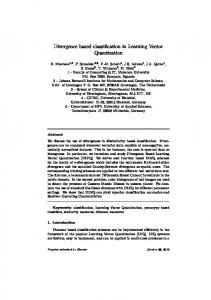
A Vector Quantization Approach for Life-Long Learning of Categories Stephan Kirstein1,2 , Heiko Wersing2 , Horst-Michael Gross1 and Edgar K¨ orner2 1

Ilmenau University of Technology Neuroinformatics and Cognitive Robotics Lab P.O.B. 100565, 98684 Ilmenau, Germany {stephan.kirstein,horst-michael.gross}@tu-ilmenau.de 2 Honda Research Institute Europe GmbH Carl-Legien-Str. 30 63073 Offenbach am Main, Germany {heiko.wersing,edgar.koerner}@honda-ri.de Abstract. We present a category learning vector quantization (cLVQ) approach for incremental and life-long learning of multiple visual categories where we focus on approaching the stability-plasticity dilemma. To achieve the life-long learning ability an incremental learning vector quantization approach is combined with a category-specific feature selection method in a novel way to allow several metrical “views” on the representation space for the same cLVQ nodes.

1

Introduction

The target of our proposed architecture is to perform supervised, interactive, and incremental life-long learning of several visual categories by combining incremental learning of learning vector quantization (LVQ) nodes with a categoryspecific forward feature selection method. Additionally we are approaching the so-called “stability-plasticity dilemma”, which occurs when neural networks are trained with a limited and changing training ensemble, causing the well known “catastrophic forgetting effect” [1]. A common strategy for life-long learning architectures (e.g. [3, 7]) is the usage of an individual node learning rate combined with incremental node insertion. This permits plasticity of newly inserted neurons, while the stability of matured neurons is preserved. The major drawback of those architectures commonly used for classification tasks is the lack of separating coocurring visual categories. This means for natural objects which typically belong to several different categories (e.g. red-white car) a decoupled representation for each category (for category red, white and car) should be learned. This leads to a compact representation and higher generalization performance compared to classification, which can’t be achieved with standard life-long learning architectures. Another approach to the “stability-plasticity dilemma” was proposed by [10]. Here representative input-output pairs are stored into a long term memory for stabilizing an incremental radial basis function (RBF) like network. Additionally it also accounts for a feature selection mechanism based on incremental principal component analysis, but no category-specific feature selection is applied, which makes it unsuitable for categorization tasks without modification.

2

Input Image

Shape Features green

...

red

0.8 0.2 0.0 0.0

Feature Vector

0.3

yellow yes blue no duck yes cup unknown

1 −1 1 0

Categories

ti

...

blue

Color Features

0.0 0.0 0.5 0.0

xi

0.4

Fig. 1. Feature extraction. Color features are extracted as histogram bins in RGB space. Shape features are obtained from parts-based feature detector. Shape and color features are concatenated into a single “flat” vector representation. The target categories are represented in a category vector ti for each feature vector xi .

The manuscript is structured as follows: in Section 2 we describe the feature extraction model using shape and color features, and introduce our category learning architecture. We show the application to a visual categorization task in Section 3 and discuss results and related work in Section 4.

2 2.1

Memory Architecture for Learning of Visual Categories Feature Extraction

Color Features. For the representation of color information we use the common histogram binning method combining robustness against view and scale changes with computational efficiency [11]. We use 6x6x6=216 histogram bins within the RGB space, where typically only a small amount of features is active. Shape Features. Our shape features are a set of preselected SIFT-descriptors defining parts-based detectors as proposed by [5]. For each new object view the response of those detectors is calculated at each location in the image using the dot product as similarity measure. The maximum response per feature detector is kept and stored in an activity vector, which neglects all spatial information. The offline feature selection scheme follows the approach described in [5], where all SIFT-descriptors of each training image are clustered into 100 components. Out of the large number of resulting clusters an iterative scheme selects at each step a SIFT-descriptor as new detector until a given number is reached (e.g. 500 in our case). The choice of detectors is independent from our category learning method and is based on the highest additional gain for a certain shape category. Combined Feature Representation. For our categorization task the color histogram and parts-based shape representation are combined into a single structureless feature vector xi = (xi1 , ..., xiF ) for each image with F = 716. Each vector xi is assigned to a list ti = (ti1 , ..., tiC ) of several color and shape categories, where each tc ∈ {−1, 0, +1} labels a xi as positive or negative example of category c.

3

The third state tc = 0 means unknown category membership and is required, because we do not assume that all category labels are provided by the tutor. Due to the nature of our feature preprocessing the data in the xi is sparse and nonnegative. For our categorization task we are particularly interested in discovering the structure from the high-dimensional feature vectors xi . Therefore we do not give the qualitative separation of the extracted features to the learning system as a priori information, but rather want to obtain a flexible metrical adaptation for the categorization. Assume you want to learn the category “fire engine”. If only shape features are used it would be difficult to distinguish this category from other cars and trucks, because the most distinctive feature, the red color, is not included in the feature representation. Therefore we let the learning algorithm decide which feature combinations are most suitable to represent a category. 2.2

Memory Architecture for Learning Visual Categories

Our memory architecture is based on a forward feature selection method combined with an incremental learning exemplar-based network to allow life-long learning of several visual categories. Both parts are optimized together to find a balance between insertion of features and allocation of nodes, while using as few resources as possible, which is crucial for interactive and online learning with respect to the required computation time. In the following we refer to this architecture as category learning vector quantization (cLVQ). The used wrapper method for category-specific forward feature selection enables the separation of coocurring categories, because it defines category specific metrical “views” on the nodes of the exemplar-based network. There are three groups of feature selection methods (see [2] for an overview). The first group are filter methods, where subsets of features are selected as a preprocessing step, independently of the chosen classifier architecture. The second group are wrapper methods, as used in our memory architecture. Here the methods use the learning architecture as a black box, to score different feature subsets, but are independent of the learning architecture. The last group are embedded methods where the feature selection process is an integrated part of the learning architecture, typically realized with sparsity constraints added to the error function. Exemplar-Based Network as Memory Architecture. The exemplar-based network part of our memory architecture is motivated from the iLVQ [7] and is extended to deal with categorization tasks. We denote the incrementally built up set of cLVQ representative vectors wk as W = {wk }k=1,...,Wn . Each wk has attached an label vector uk where ukc ∈ {−1, 1, 0} is the model target output for category c, representing positive, negative, and missing label output, respectively. Each cLVQ node wk is therefore assigned to a vector uk of several categories. For an input xi the output is determined for each category by the winning node wkmin (c) with kmin (c) = arg mink∈Ac (dc (wk , xi )), where the minimum is only determined for representatives in the set Ac = {k|ukc 6= 0} of known category-labeled vectors. The final k (c) model output is then given as oic (xi ) = uc min .

4

A key element in the cLVQ architecture is the adaptive category-specific distance computation dc that is strongly dependent on the integrated incremental feature selection process. We use a weighting of Euclidean dimensions [4] with specific weight factors λcf according to: i

k

dc (x , w ) =

F X

λcf (xif − wfk )2 .

(1)

f =1

The category-specific weights λcf are updated incrementally, which we describe in the following sections in more detail. We denote the set of active categories as C = {c}c=1,...,Cn , and the set of active features for an active category c ∈ C as Sc . We choose λcf = 0 for all f 6∈ Sc , and otherwise adjust it according to a scoring procedure explained later. The winning nodes wkmin (c) (xi ) are calculated independently for each category c. Each wkmin (c) (xi ) is updated based on the standard LVQ learning rule [8], but is restricted to feature dimensions f ∈ Sc : k

wf min

(c)

k

:= wf min

(c)

k

+ µ Θkmin (c) (xif − wf min

(c)

) ∀f ∈ Sc ,

(2)

where µ = 1 if the categorization decision for xi was correct, otherwise µ = −1 and the winning node wkmin (c) will be shifted into the opposite direction as xi . Additionally Θk is the node-dependent learning rate as proposed in [7]. The learning dynamics of the cLVQ memory architecture is organized in training epochs composed of the following steps: Step 0: Training Objects. For each epoch only a limited number of objects are visible to the architecture, emulating a limited short term memory (STM). All learning in the cLVQ network is based on the training feature inputs X = {xi }i=1,...,Xn and target category values {ti }i=1,...,Xn of these object views. Step 1: Feature Scoring Update. For the later feature selection in Step 3 we compute for each feature f and available category c a score rcf = Mf c /(Mf c + ¯ f c ), where Mf c and M ¯ f c are the number of previously seen positive and negM ative training examples respectively. For each new training example the values are updated with Mf c := Mf c + 1 for all xi with tic = +1 and xif > 0 and ¯ f c := M ¯ f c + 1 if tic = −1 and xi > 0. The score defines the metrical weighting M f in the cLVQ representation space. We thus choose λcf = rcf for all f ∈ Sc and λcf = 0 otherwise. Step 2: Initialization of Categories. If a category c with training vectors xi and corresponding category label tic = +1 occurs the first time, we initialize this category c with a single feature and one cLVQ node. We select the feature vc = arg maxf (rcf ) with the largest score value and initialize Sc = {vc }. As the initial cLVQ node for category c we select the training vector xi , where the selected feature vc is highest activated, i.e. wWn +1 = xj with xjvc > xivc for all i. n +1 = 1 and zero for all other vector The attached label vector is chosen as uW vc entries. Step 3: Feature Testing. The target of this step is the addition or removal of features for the category-specific metrics, based on the observable training set errors. For each category c we determine the set of positive errors Ec+ = {i|tic =

5

1∧tic 6= oic } and negative errors Ec−P = {i|tic = −1∧tic 6= oic }. If #Ec+ > #Ec− then P + i we compute lcf = i∈Ec+ H(xf )/ i∈Ec+ 1, where H is the Heaviside function. + The score lcf is the ratio of active feature entries for feature f among the positive training errors of class c. We want to add now a feature to the category feature set Sc , which both contributes to the class c in the training data and is very active for the encountered error set Ec+ . Therefore we choose + + rcf ) and add Sc := Sc ∪ {vc }. The added feature dimenvc = arg maxf 6∈Sc (lcf sion modifies the cLVQ metrics and we can now compute the total categorization error on the training set before and after the change. If the performance increase for category c is larger than a threshold ǫ, then vc is permanently added. Otherwise is is removed and excluded for further training iterations of this epoch. An analog step is performed, if the number of negative errors is larger than the number of positive errors (#Ec+ < #Ec− ), with the difference that the feature is removed and then again the performance gain is computed for the final decision on the removal. Step 4: cLVQ Node Testing. Similar to Step 3 we test new cLVQ nodes only for erroneous categories. In contrast to the node insertion rule proposed in [7], where nodes are inserted for training vectors with smallest distance to wrong winning nodes, we propose to insert new cLVQ nodes based on training vectors xi with most categorization errors over all categories, until for each erroneous category c at least one new node is inserted. The corresponding attached label output vector uk = ti is only filled at category positions, where category informations are available and is otherwise zero. This leads to a more compact representation, because a single node typically improves the representation of several categories. Again we calculate the performance increase based on all currently available training vectors. If this increase for category c is above the threshold ǫ, we make no modifications to cLVQ node labels of the corresponding newly inserted nodes. Otherwise we set the corresponding labels ukc of the newly inserted nodes wk to zero and remove nodes where all ukc are zero. Step 5: Stop condition. If all remaining categorization errors are resolved or all possible features f of erroneous categories c are tested, go to Step 0 and start the next training epoch. Otherwise go to Step 3 and test further feature candidates and cLVQ nodes.

3 3.1

Experimental Results Object Ensemble

For evaluating our cLVQ architecture we use an image ensemble composed of 56 different training objects and 56 distinct objects for testing (see Fig. 2), which were never used during the training phase. For each object 300 views are taken in front of a black background while rotating it around the vertical axis. Overall our object ensemble contains ten different shape categories and five different color categories (see Fig. 2). It should be mentioned that several objects

6

Fig. 2. Examples of training (left) and test objects (right) used for our categorization task, where 15 different categories are trained. As color categories red, green, blue, yellow and white are trained. The shape categories are animal, bottle, box, brush, can, car, cup, duck, phone, tool. Each object was presented in front of a black background while rotating around the vertical axis (bottom), resulting in 300 images per object.

are multi-colored (e.g. the cans) where not only the base color should be detected, but also all other prominent colors. This multi detection constraint complicates the categorization task compared to the case where only the best matching category or the best matching category of a specified group of visual attributes (e.g. one for color and one for shape) must be detected. 3.2

Categorization Results

We compare our proposed life-long learning architecture cLVQ with a single layer perceptron (SLP) and a simplified version cLVQ∗ . The SLP output for each cati c i c egory is given as oslp c (x ) = tanh(wf ∗ x − θc ), where w is a single linearly separating weight vector with threshold θc for each c. Training of the SLP consists of standard stochastic gradient descent in the sum of quadratic difference errors between training target and model output. In contrast to the more common used ROC curves we estimate the rejection thresholds during the learning process, based on the average activation strength. This is required to allow categorization of new object views at any time which is an essential requirement for interactive learning tasks. We refer to cLVQ∗ as a modified version of cLVQ, where all features without dynamic feature weighting are used, allowing conclusions about the effect of feature selection and weighting. Additionally the node performance gain threshold ǫ was set to zero. For all experiments summarized in Fig. 3 we trained the different network architectures with a limited and changing training ensemble composed of a visible “window” of only three objects, to test the life-long learning ability of our cLVQ architecture. For each epoch only three objects are visible to the learning algorithm, where at the beginning of each epoch a randomly selected object is added, while the oldest one is removed. This scheme is repeated until all 56 training objects are presented once to the network architectures. Although no prior information is given with respect to the kind of categories, we distinguish for the performance measurement between color and shape cat-

7

b) Shape Categories

Categorization Performance

1

0.9 0.8 0.7 0.6

cLVQ cLVQ* SLP

0.5 0.4 0

5

10

15

20

25

30

35

Training Epochs

40

45

50

55

0.9 0.8 0.7

8

4

0 0

5

10 15 20 25 30 35 40 45 50 55

Training Epochs

0.6

cLVQ cLVQ* SLP

0.5 0.4 0

12

d)400 LVQ Node Usage

5

10

15

20

25

30

35

Training Epochs

40

45

50

55

Number of LVQ Nodes

1

Average Selected Features

a) Color Categories

Categorization Performance

c) 16 cLVQ Feature Usage

350 300 250 200 150 100

cLVQ cLVQ*

50 0 0

5

10 15 20 25 30 35 40 45 50 55

Training Epochs

Fig. 3. Comparison of categorization performance for SLP, cLVQ∗ and cLVQ, averaged over five runs. The categorization performance is calculated after each training epoch, based on all test objects. This means that the performance is calculated based on the representation of the so far seen objects, simulating an interactive learning session. a) For the color categories the cLVQ algorithm performed better compared to the cLVQ∗ . The SLP performance is in between both LVQ approaches. b) Compared to the color categories the cLVQ∗ is slightly better than cLVQ for shape categories, while the SLP performed worst. c) Shows the number of selected features, averaged over all categories, while d) shows the allocation of cLVQ nodes during training.

egories to discuss the different quality of extracted features. The overall performance of the cLVQ architecture as shown in Fig. 3 is high for both feature modalities. For the color categories it performs much better than the simpler cLVQ∗ , while for the shape categories the cLVQ∗ performs slightly better. In general it can be said, that the feature selection method, typically selecting less than 5% of all available feature dimensions F = 716 (see Fig. 3.c), is able to capture the category information and also strongly reduces the necessary amount of required resources, which is crucial for interactive learning. Despite the fact that cLVQ typically requires only half of the nodes compared to cLVQ∗ as shown in Fig. 3.d it is even about 100 times faster. The cLVQ algorithm is even a few times faster than the SLP network, making it well suited for interactive learning. The SLP performance is surprisingly high for all trained categories. This is somehow contradictory to classification tasks, with a one-out-of-n class selection, where the SLP approach is known for the “catastrophic forgetting effect” [1]. For our categorization task this effect is only slightly visible for the shape categories. Although the forgetting effect is less present in our categorization task the SLP approach is still considerably worse than cLVQ for both feature modalities.

4

Discussion

We propose a architecture for life-long learning of visual categories, able to perform an automatic feature selection, feature weighting and incremental allocation

8

of cLVQ nodes, which is suitable for interactive learning. The wrapper method for automatic feature selection is mainly used because the representation of categories should use as few feature dimensions as possible, which can not be achieved with simple filter methods, where typically only a small amount of redundant or noisy features are eliminated. There are metric adaptation methods for LVQ networks like the GRLVQ proposed by [4] which was used by [6] as embedded method for feature selection. Those metric adaptation methods are designed for feature weighting but lack the ability to separate coocurring visual attributes and are therefore not applicable to categorization tasks. Especially this separation capability of coocurring categories combined with fast interactive and incremental learning makes cLVQ beneficial for categorization tasks. In comparison to many other categorization approaches we are able to learn multiple categories at once, while commonly the categories are trained individually. Additional many computer vision approaches dealing with categorization like the implicit shape models (ISM) proposed in [9] only uses the canonical views of the category (e.g. only side views of cars), while we rotate the objects around the vertical axis, which causes much higher appearance changes. This illustrates that our exemplar-based method can deal with a larger within-category variation, which we consider crucial for complex categories.

References 1. French, R. M.: Catastrophic Forgetting in Connectionist Networks: Causes, Consequences and Solutions. Trends in Cognitive Sciences 3 (4) (1999) 128–135 2. Guyon, I., Elisseeff, A.: An Introduction to Variable and Feature Selection. Journal of Machine Learning Research 3 (2003) 1157-1182 3. Hamker, F. H.: Life-long learning Cell Structures - Continously Learning without Catastrophic Interference. Neural Networks 14 (2001) 551–573 4. Hammer, B., Villmann, T.: Generalized Relevance Learning Vector Quantization. Neural Networks 15 (2002) 1059–1068 5. Hasler, H., Wersing, H., K¨ orner, E.: A Comparison of Features in Parts-based Object Recognition Hierarchies. Proc. ICANN (2007) 210–219 6. Kietzmann, T. C., Lange, S., Riedmiller, M.: Incremental GRLVQ: Learning Relevant Features for 3D Object Recognition. Neurocomputing (2007) (in Press) 7. Kirstein, S., Wersing, H., K¨ orner, E.: A Biologically Motivated Visual Memory Architecture for Online Learning of Objects. Neural Networks 21:65-77 (2008). 8. Kohonen, T.: Self-Organizing and Associative Memory. Springer Series in Information Sciences, Springer-Verlag, third edition (1989) 9. Leibe, B., Leonardis, A., Schiele, B.: Combined Object Categorization and Segmentation with an Implicit Shape Model. ECCV’04 Workshop on Statistical Learning in Computer Vision (2004) 10. Ozawa, S., Toh, S. L., Abe, S., Pang, S., Kasabov, N.: Incremental Learning of Feature Space and Classifier for Face Recognition. Neur. Netw. 18 (2005) 575–584 11. Swain, M. J., Ballard, D. H.: Color Indexing. International Journal of computer Vision 7 (1) (1991) 11-32