A Light-Weight Integration of Automated and Interactive Theorem

Under consideration for publication in Math. Struct. in Comp. Science

A Light-Weight Integration of Automated and Interactive Theorem Proving K A R I M K A N S O1† and A N T O N S E T Z E R2‡ {cskarim1 ,a.g.setzer2 }@swansea.ac.uk Deptartment of Computer Science Swansea University UK Received January 2011

In this paper, aimed at dependently typed programmers, we present a novel connection between automated and interactive theorem proving paradigms. The novelty is that the connection offers a better trade-off between usability, efficiency and soundness when compared to existing techniques. This technique allows for a powerful interactive proof framework that facilitates efficient verification of finite domain theorems and guided construction of the proof of infinite domain theorems. Such situations typically occur with industrial verification. As a case study, an embedding of SAT and CTL model-checking is presented, both of which have been implemented for the dependently typed proof assistant Agda. Finally an example of a real world railway control system is presented, and shown using our proof framework to be safe with respect to an abstract model of trains not colliding or derailing. We demonstrate how to formulate safety directly and show using interactive theorem proving that signalling principles imply safety. Therefore, a proof by an automated theorem prover that the signalling principles hold for a concrete system implies the overall safety. Therefore instead of the need for domain experts to validate that the signalling principles imply safety they only need to make sure that the safety is formulated correctly. Therefore some of the validation is replaced by verification using interactive theorem proving.

1. Introduction Martin-L¨ of dependent type theory offers a powerful mechanism to construct mathematical formulæ and write functional programs (Nordstr¨om, Petersson & Smith 1990); it is essentially typed λ-calculus with the dependent product and algebraic data-types. By the Curry-Howard correspondence (Curry 1934, Curry, Feys, Craig & Craig 1958, Howard † ‡

Partly supported by Invensys Rail Systems, UK. Supported by EPSRC grant EP/G033374/1, theory and applications of induction-recursion. Part of this work was done while the second author was a visiting fellow of the Isaac Newton Institute for Mathematical Sciences, Cambridge, UK.

Kanso and Setzer

2

1980), propositions can be represented as types, where an element of the type is a proof of the proposition. Another perspective in type theory is that a type is a specification of a problem such that its elements are programs that satisfy the specification. In this paper, we investigate and actualise an embedding of automated theorem proving (ATP) decision procedures into Martin-L¨ of dependent type theory. The motivation is twofold. The first one is to integrate Agda (Bove, Dybjer & Norell 2009) with fast external tools that facilitate feasible verification of large finite problem sets, archetypal of industrial verification. Secondly we want to explore a functional proof framework where finite (or finitisable) components of a theorem are proved automatically and the infinite components are proven with human guidance. Mature proof assistants such as Isabelle and Coq have supported external tools for many years (B¨ ohme & Nipkow 2010, M¨ uller & Nipkow 1995, Boutin 1997), whereas Agda, a less mature tool, does not yet. The fact that Agda is quite new has provided an opportunity for the community to experiment with new approaches (some official and some not) regarding many theoretical aspects of Interactive Theorem Proving (ITP) tools. The new approaches taken in Agda have resulted in it being an intuitive proof assistant which is also a programming language; programs and proofs are defined using the same functional constructs that can be compiled and executed. We believe that Agda can be extended into a platform for the development of verified software. Our wider ambition is to have a substantial program (such as a critical system with hundreds of variables) which executes in Agda and is proven to be correct with respect to safety in the target domain. We have realised this ambition with a number of train control systems, the largest system containing ≈ 600 propositional variables, and will give full details about a smaller example (Section 5). In this scenario, concrete finite domain theories need to be proven to show the system satisfies some properties, and abstract infinite domain theories need to be proven that show correctness of the properties and verification techniques. One example, where the combination of finite domain theorems proved using ATP and infinite domain theorems proved using ITP is of great benefit, is the reduction of the problem of domain validation. We will give two case studies of how to carry this out in Sections 4 and Section 5. Consider the development of a critical system that must satisfy a number of safety conditions which are lemmata from the target domain. Informally safety conditions are rules-of-thumb that are used by developers and testers of critical systems. One can prove using ITP that these safety conditions imply the actual “safety” of the system, where the concept of “safety” still remains to be validated by domain experts, and is expressed as a theorem over infinite domains. For instance, within the train domain where the safety conditions are synonymous with signalling principles, it is possible (depending on the precise set of signalling principles in use) to prove they imply that “trains do not collide or derail”. So instead of validating all the safety conditions, some of them have been verified. It might be the case that the safety conditions are insufficient to guarantee safety, or that some are redundant or worse, contradictory. Thus part of the validation procedure (done by domain experts) has become a verification procedure (done by mathematicians), which reduces the total amount of validation required and increases trust that the system is safe. Then as a

Mathematical Structures in Computer Science

3

concrete step, we develop in Agda and verify with (possibly certified) ATP tools that the system satisfies the safety conditions. Thus the actual “safety” of the system has been shown (in Agda) to follow from the safety conditions, not only that the system satisfies the safety conditions. In this work it is not essential (but complimentary) that the ATP tools are certified, it is however recommended that the tools are well-established and widely trusted within the ATP/verification communities. 1.1. Related Work Since N. de Bruijn introduced AUTOMATH in the late 1960’s (de Bruijn 1970), the ITP community has studied the issue of automatically solving problem sets many times (Bierman, Gordon, Hrit¸cu & Langworthy 2010, B¨ohme & Nipkow 2010, Boutin 1997, Fontaine, Marion, Merz, Nieto & Tiu 2006), and many more. We have during this research identified three existing approaches for integrating automated and interactive theorem proving, none of which categorises our approach. Oracle. The use of an oracle, which is an operation that provides a proof of a theorem, and which when invoked calls an external tool. See for instance approaches by Owre and Rush in PVS; Tverdyshev, M¨ uller and Nipkow in Isabelle; and Bierman, Gordan and Langworthy in M (Owre, Rushby & Shankar 1992, M¨ uller & Nipkow 1995, Bierman et al. 2010). There are too many interactive tools to list that use external tools as oracles, but relevant to this project is the RODIN tool set (Abrial, Butler, Hallerstede & Voisin 2006) which is similar to PVS in that it tries to help system developers write verified software. The problem with this approach is that the result of the oracle does not reduce to head normal form, and therefore destroys the ability to execute programs. Another problem is that it is not clear whether the external tool is correct and whether the result of the external tool was interpreted correctly. Reflection. The correctness of a decision procedure is verified in the ITP tool, and from this proof a verified ATP tool (Boutin 1997) is extracted. The extracted program is called by a tactic to build a proof. This approach has for instance been taken by Verma; Hendriks; and Lescuyer and Conchon (Verma 2000, Hendriks 2002, Lescuyer & Conchon 2008), and has been widely applied within the Coq community. Reflection requires a correctness proof for an ATP tool in the ITP tool; proving the correctness for state-of-the-art theorem provers would be cumbersome and one would expect the stat-of-the-art tools to have significantly improved by the time the proof is complete. Oracle with Justifications. One uses an ATP tool which provides in case of a positive answer a proof-object (Diller & Troelstra 1984), which can then be translated automatically into an ITP proof of the corresponding ITP formula. Since the ITP proof is now checked, the correctness relies entirely on the correctness of the ITP checker. Furthermore, a proof-object is kept and therefore the ATP has to be executed only once. This approach has been used for instance by (Paulson & Susanto 2007, B¨ohme & Nipkow 2010, Dong, Ramakrishnan & Smolka 2003, Weber 2006, Fontaine et al. 2006). Notably Simon Foster has used this technique to connect Agda with Waldmeister (Foster & Struth 2011). Problems are that creating the proof-object slows down the ATP tool, and that many ATP tools do not provide a proof-object. Further-

Kanso and Setzer

4

more the proofs provided by the ATP tool might be very big (proof sizes of several hundreds of Megabytes have been reported for Satisfiability Modulo Theories (SMT) solving (Stump 2009)). Therefore checking translated ITP proofs might be infeasible, especially when dealing with type theoretic ITP tools. This is due the size of the proof terms and garbage collection issues. Remark: It should be noted that the paradigms of oracles, and oracles with justifications have been identified as far back as 1970 (de Bruijn 1970). A good introduction to the various different flavours of theorem proving can be found in (Harrison 2008), and a more technical discussion in (Boutin 1997). A review of formal methods relating to industrial projects can be found in (Woodcock, Larsen, Bicarregui & Fitzgerald 2009).

1.2. Our Approach – Oracles & Reflection Assume a logic (such as propositional), define the set of formulæ and a satisfaction relation with respect to the logic. Then the decision procedure is implemented in Agda’s logic with the focus on an easy proof of correctness rather than efficiency (in fact the implementation could be na¨ıve and highly inefficient). It is then proved to be correct with respect to the satisfaction relation. In Agda, a function’s implementation can be overridden by a native Haskell implementation (after checking that the function fulfils a number of axioms); using this fact, the inefficient decision procedure is replaced by a call to an external ATP tool. Evaluation of the decision procedure is as follows: if applied to a closed term, the efficient ATP tool is executed; if applied to an open term, the na¨ıve (inefficient) Agda implementation is evaluated. Since the correctness proof refers to open terms, it refers to the Agda implementation and not the ATP tool. If the resulting proofobject is inspected, it is lazily evaluated using the na¨ıve implementation; otherwise it behaves as if it has been postulated. In order to make sure that the native implementation is used correctly, we make sure that the input language of the overridden function is an Agda representation of the input language of the tool. If the original problem requires a translation into this input language, then we define the correctness of the problem in the input language of the tool, and a translation of the original problem into this input language. Then we prove that if the correctness of the problem related to the input language holds, then the correctness of the intended original problem holds as well. Therefore the translation is provably correct. An example is CTL model-checking (see Section 2.4), where the transition relation is made total before executing the external tool. The function overridden requires that the transition relation is total. The problem for the non-total transition relation is inside of Agda reduced to this situation. To increase trustworthiness, the input and outputs of the ATP tool are logged, allowing a user to manually verify the translation and the tool’s result are correct. Our approach yields a high-level of soundness and efficiency when using certified ATP tools. See Section 2.2 for technical details on the embedding and Section 1.3.1 for a discussion of the soundness.

Mathematical Structures in Computer Science

5

1.3. Comparison with Existing Approaches Obviously, compared with only using an oracle the approach has the advantage that proofs normalise and programs can be extracted. Both the oracle and our approach become inconsistent if the result of the external tool is incorrect, see Lemma 2.1. Pure reflection has the highest level of soundness of all approaches as no external tools are used. In comparison, our approach, in the case of open terms is equivalent; but in the case of closed terms weakens soundness and significantly increases efficiency. The third approach where the external ATP tool provides a justification is motivated by the fact that in many cases, non-trivial translations into the ATP tool’s input language are defined outside the logic of the ITP tool, making it hard to prove that they preserve correctness (Fontaine et al. 2006). Instead with our approach these translations are defined inside Agda, mitigating this requirement. It follows from this that in our approach the tools do not need to compute justifications, and hence the tools can be more efficient, and the choice of tool is less restrictive. The ATP tool can range from unverified state-of-the-art tools to certified but technologically less advanced tools. In summation, we trade the high-level soundness assurances that justifications provide for an increase in efficiency, flexibility and usability; this soundness trade-off is minimal when using certified external tools. Also in our approach there is no need for the ITP tool to store and check the justifications. One should as well note that whatever we do in order to guarantee the correctness of proofs carried out using ITP, we can never obtain absolute certainty. We will always rely on the correctness of the checker of theorems in the ITP (which are usually not formally verified), and on the correctness of its logic (most ITP tools substantially deviate from the underlying logical theories in order to be more user friendly). Then we rely as well on the correctness of the compiler (it is well known that most compilers have errors) used to compile the ITP tool, and on the underlying operating system. And ultimately G¨odel’s incompleteness theorem shows that it is impossible to guarantee that the underlying mathematical theory is consistent.

1.3.1. Soundness. This approach is sound, provided the ITP tool (Agda) is sound and the ATP tool gives the correct output, which means that it returns true, if the formula to be proved is valid, and false if it is not. The reason is that one shows in Agda that the inefficient function which is to be overridden, fulfils this property. Since there is only one such function, the overridden function returns the same result as the original inefficient function defined in Agda. So Agda with the function overridden is equivalent to Agda without it, and if the latter is sound, so is Agda with the overriding mechanism. The logging of the answers of the ATP tool gives the user the possibility to check whether the instances used the ATP tool gave the correct answer (e.g. by checking using alternative tools), and therefore reduces the reliance on the soundness of the ATP tool. We note as well that the input to the ATP tool will be done in the language of the ATP tool (using a syntactic representation in Agda). The translation of the original problem into the ATP tool’s input language is done inside Agda, and therefore shown to

Kanso and Setzer

6

be correct. This avoids the problem of an erroneous translation, which might for instance happen if the translation is carried out by a program outside Agda. We think as well that many ATP tools are at least as trustworthy as Agda itself (if not even more), so this approach won’t weaken the correctness of Agda. 1.3.2. Intuitionism and Classic Provers. We note that the use of SAT solvers based on classical logic are compatible with the intuitionistic type theory of Agda: the SAT solver is only applied to formulæ formed from decidable prime formulæ (e.g. formulæ of the form T (b) for a Boolean term b), for which the principle of tertium non datur holds intuitionistically. The principle of tertium non datur holds for all propositional formulæ, provided it holds for the atomic formluæ this formula is built of, so for these formulæ classical logic holds in intuitionistic type theory. In the case of CTL, one can show as well the principle of tertium non datur, provided it holds for the atomic formulæ it is built from. In fact the decidability of the validity of formulæ expresses that tertium non datur holds. Therefore any theory with decidable validity fulfils tertium non datur.

1.4. Overview Section 2.1 provides a comparison of automated and interactive theorem proving techniques and an overview of finite and infinite theories, Section 2.2 introduces the technique used for embedding ATP theories into type theory. Section 2 then concludes with two examples of the embedding, the first example being Boolean tautology checking, and the second example being Computation Tree Logic (CTL) model-checking in Section 2.3 and Section 2.4, respectively. Section 3 discusses how Agda was extended to allow for the technique described in this paper. This entailed extending the type-checker to check the decision procedures against axioms and low-level interfacing of the external ATP. Furthermore, a generic plug-in interface is described in Section 3.1. Sections 4 & 5 provide two examples of the composition with respect to specifying, developing, and verifying control systems for specific domains. We give an abstract notion of safety, and show using ITP that safety conditions (in railways called signalling principles) imply this safety. Then we verify using ATP that the safety conditions hold for a concrete implementation, and therefore obtain overall safety of these implementations. Finally, Section 6 summarises the paper and presents the concluding remarks.

2. Methodology In this section we discuss the advantages and disadvantages of automated and interactive theorem proving, and present a general technique of embedding automated theorem proving theories. This is concluded with two examples of the embedding, namely Boolean tautology checking and CTL model-checking.

Mathematical Structures in Computer Science

7

2.1. Comparison of Automated and Interactive Theorem Proving Techniques Generally, theorem proving tools can be placed into one of two categories, interactive or automatic (Boutin 1997). The first category, ATP tools attempt to prove a theorem by automatically deducing the proof from already proven lemmata. In some cases, intermediate lemmata are introduced and proven automatically. The user has no direct influence over the derivation and proving process. In this work, only ATP tools that coincide with decision procedures for logics are considered as they are admissible intuitionistically; examples are SAT solving and model-checking. Conversely the second category is formed by ITP tools, i.e. proof assistants or proof checkers; they work by allowing the user to guide the derivations and proofs of lemmata, culminating in a proof of the desired theorem. 2.1.1. ATP tools are very powerful when dealing with concrete theorems over finite domains as in SAT and finitisable domains as with temporal logics. In some cases ATP tools can be applied to theorems over infinite domains as in SMT (Barrett, Sebastiani, Seshia & Tinelli 2009) and first order provers, but this class of tools typically become semi-decidable decision procedures (De Moura & Bjørner 2009) and are not considered in this work. Industrial hardware and software verification is archetypal of finite concrete theorems – large but not inherently complex problems†. ATP tools often allow the system to be modelled using an intuitive language, and the desired properties of the system to be specified in the tool’s logic. The tool will attempt to prove these properties, when this is not possible the tool will either provide a counter-example of the property or declare an unknown result. These unknown results typically occur as a result of attempting to prove a theorem that has an infinite component and not knowing which lemma to apply or when a resource (time or space) is not sufficient to complete the proof. 2.1.2. ITP tools are powerful when dealing with theorems over infinite domains for which it is not known (at least currently) how to mechanise their proofs. Consider a theorem of the form ∀n.ϕ in which ϕ has an infinite component. It could be possible to prove it using standard induction, but often the theorem needs to be strengthened such that the new theorem ∀n.ϕ ∧ ψ implies the desired theorem. The choice of this strengthened theorem, in general requires input from a human being. The reason is that when proving the inductive step, ϕ(n) might not be sufficient to imply ϕ(n + 1); whereas a stronger theorem ϕ(n) ∧ ψ(n) might be sufficient. To choose ψ such that it is strong enough to allow the theorem to be proved without being so strong that it hinders the proof is a complex task and cannot be mechanised in general. ITP tools have the advantage that unknown results do not occur as the user guides the proof and the tool checks that the proof is correct. 2.1.3. Limitation of using ATP alone. As an example, consider a simple reactive system realised using Boolean valued equations which compute the next state from the current state and input variables. The most natural way to verify such a system is †

We refer to this type of verification as industrial.

Kanso and Setzer

8

using SAT based verification. Assume a safety‡ property P . One would have to construct the propositional formula which expresses that P holds in all reachable states, i.e. ∀reachable state s.P (s). For small state spaces it is possible to enumerate all states and take their conjunction, but for realistic systems this is not feasible§ . Therefore the fastest method to determine whether the system models P is to apply induction. This would yield two proof obligations which take into account reachable states, namely the base case (initial state) and inductive step (transition function). After the user has entered these into a SAT solver and determined validity of both cases, there is still a meta-step to be performed by the user. The meta-step here is to prove validity of induction outside the SAT solver. The user can then assemble the three proofs to determine that P always holds in all reachable states. SAT solving alone is not sufficient to efficiently prove this theorem. This example, perhaps contrived, shows the limitation of ATP alone, and in general this final task of assembling proofs is more complicated. See Sections 4 & 5 for substantial examples where various ATP proofs are assembled to show that a road crossing and a railway interlocking system are safe. When using ITP tools on large finite concrete theorems the work delegated to the user is exorbitant (Jones, Grov & Bundy 2010). Industrial verification is a special case where large numbers of mechanisable, and a small number of un-mechanisable proof obligations arise (Woodcock et al. 2009). It would be nice to use ATP tools for the mechanisable proof obligations. The next section discusses our embedding of ATP theories into type theory to mitigate the user’s work-load.

2.2. General Technique The embedding of a chosen ATP theory into type theory is as follows. Assume a logic L, e.g. propositional logic, CTL or modal-µ calculus, that the chosen ATP theory is defined over. Formulæ in L are inductively defined types, whose elements are finite. These formulæ can usually only hold with respect to a model M and an environment ξ. In this work, the model is what is fixed and does not change and the environment is what varies. For example, in CTL model-checking (see Section 2.4) the model is a transition system and a state; the environment is an infinite run of the transition system from the state identified in the model. In SAT (see Section 2.3) there is no model, but the environment assigns Boolean values to variables in the formula. In the case of first order theorems the model consists of the semantics of the signature and the environment is an assignment to variables in the formula. For technical reasons, the model and environment are defined first as the formulæ can depend upon these structures. It is now possible to give semantics to these formulæ by defining a satisfaction relation

‡ §

A safety property is a property that must hold in all reachable states. Consider a system with 600 state variables (not uncommon within industrial applications), there would be 2600 conjuncts which is larger than the number of atoms in the observable universe.

Mathematical Structures in Computer Science

9

that assigns types to formulæ with respect to M and ξ. J ⊧ K ∶ Model → Formula → Environment → Set The decision procedure DecM ∶ Formula → Bool for the ATP theory is formalised as a function. In our experience an inefficient simplistic definition that recurses over the structure of the formula, model and environment is preferable as this helps with proving correctness of DecM . Correctness of DecM is then a proof of DecM (ϕ) ⇔

∀ ξ.J M ⊧ ϕ Kξ ∃

where the choice of quantification depends upon the ATP theory. E.g. in the case of the Boolean satisfiability problem, we have “there exists a satisfying assignment” (satisfiability testing) or “all assignments are satisfying” (tautology checking). It is possible to define more complicated quantification schemes, whereby the environment is split into sub-environments; but this is not considered in this work. The proof of correctness is then used to prove theories of the form ◻ξ.J M ⊧ ϕ Kξ where ◻ ∈ {∀, ∃} by transferring the proof of the Boolean valued result of DecM (ϕ) generated by the ATP theory. The type theoretic implementation of DecM is typically inefficient compared to purpose written tools, because DecM is defined na¨ıvely to simplify the correctness proof. This inefficiency is exasperated by many implementations of proof systems; specifically relating to this work, type systems make heavy use of rewriting and normalisation resulting in large terms which would consume vast resources in attempting to evaluate DecM on all but the simplest examples. For this reason, we replace DecM with an actual ATP tool for an efficient implementation. See Section 3 for more information regarding the implementation. In order to obtain consistency, the ATP tool overriding type theoretic implementation of DecM needs to be consistent with the decision procedure. Therefore most examples of semi-decision procedures are excluded, since a na¨ıve implementation and an actual ATP tool would usually differ on, when to return an undefined result. A precise formulation of this fact is given in the following lemma: Lemma 2.1 (Built-In Consistent). Assume a function f ∶ A → B is overridden by an implementation f ′ ∶ A → B such that the following holds: — If there is a closed term a ∶ A and a defining equation of f of the form f a = b then b = f ′ a; — For at least one element a ∶ A, f a returns a different result from f ′ a. Then the resulting type theory is inconsistent. Remark: Note that if a function f ∶ A → B has a defining equation of the from f a = b for some closed a ∶ A, and it is overridden by f ′ with f ′ a = b′ , then f a will always evaluate to b′ and we don’t have access to the defining equation f a = b any more. Proof. Let f ′′ be a function of type A → B, which is defined in Agda by using the

Kanso and Setzer

10

same case distinction as f , however at the right-hand side by referring to f rather than recursively calling f ′′ . By using the same case distinction as f for f ′′ , it follows immediately that we can prove in type theory ∀x ∶ A . f x = f ′′ x (since for open terms a the definition of f is not overridden, and for closed terms a we have that f a and f a′ coincide). Let a ∶ A be such that the original value of f a differs from f ′ a. In the recursive evaluation of f a there must be a term a′ (which can be a itself) such that f a′ is evaluated incorrectly by the tool, but all recursive calls used in evaluating f a′ are evaluated correctly. Therefore f ′′ a returns the result of the non-overridden function f , whereas evaluating f a′ returns a different result (because it is being overridden). We obtain that f a′ ≠ f a′ , contradicting ∀x ∶ A . f x = f ′′ x. The technique presented here is generic and abstract; it does not only apply to type theoretic applications but generally within combining mechanised and un-mechanised mathematics. To solidify the above technique two examples are presented, Boolean tautology checking and CTL model-checking in Section 2.3 and Section 2.4, respectively. 2.3. SAT In this work, standard Boolean satisfiability is not applied; instead tautology testing of a Boolean valued formula with variables is explored, which is an equivalent problem. Tautology checking was chosen over satisfiability testing because SAT verification typically relates to checking safety properties, that is, that something undesirable will never happen. In the case of SAT the model contains no information, and for completeness it is the canonical element from a singleton set. The environment assigns Boolean values to the variables in the formula. Before introducing the definition of Boolean formulæ with variables, the notion of finite sets are introduced as they index the variables. Finite, or enumeration sets, Fin ∶ (n ∶ N) → Set are finite sets with n distinct elements, namely Fin n ∶= {0, . . . , n − 1}; notably Fin 0 = ∅. Boolean formulæ are defined as follows: data BooleanFormula (n ∶ N) ∶ Set where const ∶ Bool → BooleanFormula n var ∶ Fin n → BooleanFormula n ¬ ∶ BooleanFormula n → BooleanFormula n ∧ ∨ ⇒ ∶ BooleanFormula n → BooleanFormula n → BooleanFormula n where the underscores ( ) denote syntactic positions of required arguments. In the following we write xn for (var n). The semantics a of BooleanFormula with respect to an environment is J K ∶ ∀{n} → BooleanFormula J const b Kξ = T b J xi Kξ = ξ i J ¬ϕ Kξ = (JϕKξ ) → ∅

n → (Fin n → Bool) → Set J ϕ ∧ ψ Kξ = JϕKξ × JψKξ J ϕ ∨ ψ Kξ = JϕKξ + JψKξ J ϕ ⇒ ψ Kξ = JϕKξ → JψKξ

Mathematical Structures in Computer Science

11

To define the decision procedure, assume a function instantiate ∶ BooleanFormula (suc n) → Bool → BooleanFormula n that instantiates all occurrences of x0 with the second (Boolean valued) argument; all other variables are shifted down by one, i.e. xn+1 ↦ xn . The decision procedure for tautology checking a BooleanFormula n is defined na¨ıvely rather than using (Davis, Putnam & Robinson 1961). The reason is that it simplifies the correctness proof. It is defined by 2n applications of instantiate, then canonically with respect to the Boolean connectives. tautology ∶ ∀n → BooleanFormula n → Bool tautology zero (const b) = b tautology zero (¬ ϕ) = ¬(tautology ϕ) tautology zero (ϕ ◻ ψ) = (tautology zero ϕ) ◻ (tautology zero ψ) tautology (suc n) ϕ = tautology n (instantiate ϕ true) ∧ tautology n (instantiate ϕ false) where ◻ ∈ {∧, ∨, ⇒}. A proof of correctness is then an element of: ∀n . (ϕ ∶ BooleanFormula n) → ( T (tautology n ϕ) ↔ ((ξ ∶ Fin n → Bool) → J ϕ Kξ )) which is proven by simple induction over n. The above embedding of Boolean tautology checking has been implemented in Agda requiring 39 lines of code for the decision procedure and associated definitions (including natural numbers and Booleans). The proof of correctness requires an additional ≈ 100 lines of code which includes many basic lemmata about products, sums and the functiontype (Curry-Howard isomorphism). The decision procedure is then overridden by a call to an external SAT solver. See Section 3.2 for a discussion of the results. The code can be downloaded from the project home page (see Section 6).

2.4. CTL Model-Checking One aim of this work is to use Agda to develop and verify control systems for safety and liveness properties. To this end we have outlined a process of embedding CTL modelchecking of finite-state machines. When dealing with theorems which have substantial structure, such as model-checking that is defined over a transition system, it is important to choose definitions that simplify the embedding process. The transitions systems used here are finite and can deadlock, i.e. the transition relation is not total. Finite-state machines (FSM) are the transition systems used in this work. They are defined by the number of states, the number of atomic propositions, an initial state, a transition relation between states and a labelling of the states. The transition relation is given by two functions: arrow which determines for each state the number of transitions from it, and transition which determines for each state and arrow from this state the

Kanso and Setzer

12

successor state. data FSM ∶ Set where fsm ∶ (state atom ∶ N) → (arrow ∶ Fin state → N) → (initial ∶ Fin state) → (transition ∶ (s ∶ Fin state) → Fin (arrow s) → Fin state) → (label ∶ Fin state → Fin atom → Bool) → FSM The model of the CTL model-checking is a pair consisting of the transition system M and current state s0 . The environment (under combined operators) is an infinite run < s0 , s1 , ... > rooted at the current state s0 . Note that the current state s0 is fixed and runs starting in s0 are what are quantified over. The runs are defined by means of a co-algebraic data-type. data RunM (s ∶ Fin stateM ) ∶ Set where next ∶ (a ∶ Fin (arrowM s)) → ∞ RunM (transitionM s a) → RunM s where ∞ prefixes a term that can potentially be unfolded infinitely many times. In Agda, co-algebraic types are represented using the built-in postulated function ∞. In the following, we write runi for the ith state in run = < s0 , s1 , ..., si , ... >. π is used for finite paths and πi is the ith state in π. CTL formulæ can be defined over the model using a minimal set of combined CTL operators (Huth & Ryan 2004). EX - exists next, EG - exists globally, E[ U ] - exists until and P - state proposition.

data CTL (M ∶ FSM) ∶ Set where false ∶ CTLM ¬ EX EG ∶ CTLM → CTLM ∨ E[ U ] ∶ CTLM → CTLM → CTLM P ∶ Fin atomM → CTLM where atomM is atom projected from M. The semantics of a CTL formula is as follows: false, ¬ and ∨ are the same as in propositional logic. P a has the meaning that atomic proposition a holds in the current state. The remaining cases specify properties about infinite runs of the transition system rooted at some state s. Exists next (EX ϕ) holds when there exists a run run from s such that ϕ holds at run1 . Exists globally (EG ϕ) holds when there exists a run from s such that at each point i on the run, ϕ holds. Exists until (E[ϕ U ψ]) holds when there exists a run from s such that there exists a point k where ψ holds, and for all points j < k, ϕ holds.

Mathematical Structures in Computer Science

13

The semantics of a CTL formula with respect to a model is J , ⊧ K ∶ (M ∶ FSM) → (Fin stateM ) → CTLM → Set J M , s ⊧ false K = ∅ J M ,s ⊧ ¬ϕ K = J M ,s ⊧ ϕ K → ∅ J M ,s ⊧ ϕ ∨ ψ K = J M ,s ⊧ ϕ K + J M ,s ⊧ ψ K J M , s ⊧ P a K = T (labelM s a) J M , s ⊧ EX ϕ K = ∃ (run ∶ RunM s) J M , run 1 ⊧ ϕ K J M , s ⊧ EG ϕ K = ∃ (run ∶ RunM s) (∀i J M , run i ⊧ ϕ K) J M , s ⊧ E[ϕ U ψ] K = ∃ (run ∶ RunM s) ∃ (k ∶ N) ((∀j < k J M , run j ⊧ ϕ K) × J M , run k ⊧ ψ K) where labelM is label projected from M. Here the environment (RunM s) is existentially quantified. Determining whether a CTL formula holds in the Boolean operator cases is canonical with respect to the operators and not discussed further. The decision procedure for the first substantial operator, EX ϕ (exists next) does this by searching for a path of length stateM +1 and verifying that ϕ holds at the second point, i.e. there exists a successor state where ϕ holds. The argument for correctness of this procedure is a simpler case of correctness for exists globally, and follows by Lemma 2.2 (see below ). In the case of EG ϕ (exists globally), an infinite run is required such that at each point on this run, ϕ holds. Na¨ıvely checking each point on this run would take an infinite amount of time, thus we finitise the problem. The pigeonhole principle¶ (Dedekind 1863) (which is the principle underlying the proof of the pumping lemma (Bar-Hillel, Perles & Shamir 1964)), and the finiteness of the transition system allow the decision procedure for EG to check for a finite path of fixed length from the state s such that ϕ always holds. If a path π of length stateM +1 exists from s such that ϕ holds at each point, then it can be extended infinitely many times into a run. This follows by Lemma 2.2 (see below ). Remark: The proofs of Lemmata 2.2 & 2.3 are given in detail since the Agda representations are essentially the same proofs. Lemma 2.2 (M, s ⊧ EG ϕ). Assume a finite transition system M with n states. There exists an infinite run from state s such that ϕ holds at each point iff there exists a path π of length n + 1 from state s such that ϕ holds at each point on π. Proof. ⇒ An infinite run where ϕ holds at each point can be truncated to a path of length n+1. ⇐ By the pigeonhole principle, at least one state has been repeated in π, i.e. ∃(0 ≤ i < ¶

The pigeonhole principle states: if you put n things into m boxes where n > m, then there exists at least one box that contains more than one item.

Kanso and Setzer

14

j ≤ n) . πi = πj . Therefore a (possibly trivial) loop in the transition system exists containing πi , this loop can be repeated infinitely many times, and we obtain an infinite run.

In the case of exists until, things are a little more complicated. E[ϕ U ψ] means there exists an infinite run run such that at some point k in the future ψ must hold, but up to and not including that point, ϕ must hold. Intuitively, the decision procedure checks for a path π ϕ with length ≤ stateM such that ϕ holds at each point, and then checks for a path π ψ of length stateM +1 starting at the end of π ϕ such that ψ holds at π1ψ . This follows by Lemma 2.3. Lemma 2.3. Assume a finite transition system M with n states. M, s ⊧ E[ϕ U ψ] holds iff there exists a path π ϕ with length ≤ n from the state s such that ϕ holds at each point of π ϕ , and there exists a path π ψ of length n + 1 such that the end of π ϕ equals the beginning of π ψ and ψ holds at π1ψ . Proof. ⇒ There exists a point k on the infinite run run, such that for all points j < k, ϕ holds and at point k, ψ holds. We show that π ϕ and π ψ exist by induction on k: case k ≤ n: We are done, π ϕ is a prefix of the run, and π ψ equals the succeeding n + 1 states from k. case k > n: By the pigeonhole principle there exists two points 0 ≤ l < m < n + 1 such that run l = run m . Therefore a loop exists before point k, this loop can be removed such that ϕ holds up to point k − (m − l) and ψ holds at point k − (m − l). Let run ′ be the resulting run. By the induction hypothesis and run ′ , the assertion follows. ⇐ By Lemma 1, path π ψ can be extended infinitely many times, thus an infinite run can be constructed consisting of π ψ extended infinitely many times concatenated to π ϕ . As ϕ holds along π ϕ , and ψ holds at π1ψ , the infinite run satisfies ϕ until ψ.

The decision procedures for EX, EG and E[ U ] can be implemented by bounded traversals of the transition system and taking disjunctions between choice points in the traversals. Our implementation requires ≈75 lines of Agda code; this includes the definitions of Booleans, natural numbers, finite numbers, transition system, CTL formulæ and the decision procedure. The proof of correctness requires > 1000 lines of code because this includes the proof of the pigeonhole principle (≈ 300 lines of code) and many lemmata reasoning about finite sets and the transition system. 3. Implementation So far, everything presented has been fully contained in the ITP tool’s logic, but in practise evaluating these decision procedures is inefficient when compared to purpose written ATP tools. Generally this is because ITP tools are interpreters which result in a

Mathematical Structures in Computer Science

15

layer of abstraction between program and the hardware. Specifically in the case of Agda, this is because mechanisation of a type system looses the low-level procedural access (such as fast arrays and bit flipping operations) to the computer needed for efficient implementations. Another reason is that the decision procedure written in the ITP tool is chosen to be simple but inefficient, in order to facilitate the proof of its correctness. For this reason, we customised the ITP and programming language Agda to allow for the type-checker to call external ATP tools in-situ of evaluating the decision procedures. This involved extending the existing built-in mechanism to execute external tools (in addition to executing Haskell functions). Both of the examples presented in this paper have been fully implemented in Agda. Two branches of the Agda source were taken, one for SAT and the other for CTL. Each of these branches were customised by providing translations between Agda terms representing the problem set and the tool’s input language, an axiom check of the decision procedure and the file path to the external tool. The axiom checks guarantees that the overridden Agda function is defined correctly. The external tools are wrapped by a script that parse the output, and determine a Boolean valued result (or, if parsing fails, raises a type-checking exception) which is transferred back to Agda. Then as a final step, within Agda we provide the necessary definitions from Section 2.2 such that they pass the axiom check. These two branches provide a significant level of soundness from the end-users perspective as the user cannot modify the definition of the decision procedure as it would then fail the axiom check and raise a type-checking error; nor can the user change the external tool that is executed as it is hard-coded. These branches required a significant amount of effort to implement as knowledge of Agda’s internals is required. To simplify the process of connecting Agda to an external tool, we devised and implemented a third branch of Agda’s code that provides a generic plug-in interface for executing external tools. It should be noted that this interface trades soundness (a normal user can break the system) for usability (no re-compilation of Agda required). 3.1. Plug-in Interface We have modified Agda by adding six tags to the type-checker. Definitions in the plugin (Agda source file) can then be tagged. The internals of the type-checker can, while type-checking subsequent terms, reference a tagged definition by name. The first tag ATPProblem tags something in Set which corresponds to the problem set that the decision procedure is defined over. The second tag ATPInput depends upon the first tag, and tags a function of type ATPProblem → String that translates the problem into a string that is passed to the external tool. The third tag ATPTool tags a string which is a path to the external tool; and the fourth tag, ATPDecProc tags the actual decision procedure which must be of the type ATPProblem → Bool. The plug-in mechanism will not be activated until a proof of correctness has been provided; the final two tags, tag the semantic relation and a proof of correctness. The intuition behind these final two tags is that they force the user to prove that the provided decision procedure implements their chosen ATP theory. Typically this step of proving

Kanso and Setzer

16

will ensure that the user has thought about what it is they are doing, hence mitigating the risk of providing the wrong external tool for their chosen ATP theory, e.g. entering a SAT solver in-place of an SMT solver. This does not prevent a malicious user breaking the system, nor preventing the use of an inconsistent tool. When the function tagged by ATPDecProc is reduced on γ ∶ ATPProblem, the typechecker will execute the external tool pointed to by ATPTool. But, it first applies the function tagged by ATPInput to γ that yields a string in the tool’s input language. The Boolean valued result is computed by examining the return value of the tool. Should the tool return 0 a true value is used, should the tool return 1 then false is used; any other value results in an exception being raised and the tools output dumped into the log. These values were chosen to conform to POSIX standards. Typically it is required to write a wrapper script for the external tool that parses the output of the tool and sets the return values accordingly. We have successfully re-implemented the SAT and CTL interfaces within this generic plug-in framework, by replacing the axiom check with a proof of correctness. In terms of flexibility, this approach is very powerful as it has allowed us to extend with minimal effort the CTL interface to provide symbolic CTL. Then we extended the symbolic CTL to a customised temporal logic that is defined over ladder logic programs (IEC 611313). Therefore when executing the model-checker the original structure of the program is preserved (instead of computing its transition system). The correctness proof is given by the composition of the correctness proofs of CTL and symbolic CTL model-checking. 3.1.1. Type-Checking Justifications. Checking justifications produced by external tools is possible (and has been experimentally implemented for SAT) in this generic framework by tagging a function that takes a proof-tree generated by the external tool, and constructs a proof-object from it. When the function is evaluated on a proof-tree, the type-checker is triggered, and it checks that the proof-tree is correct with respect to the necessary inference rules. This function then implicitly overrides the soundness proof for closed terms using the same mechanism that the external tool overrides the decision procedure. This is the same approach taken by (Armand, Gr´egoire, Spiwack & Th´ery 2010) in Coq where refutation traces are type-checked using reflexive methods. According to Section 1.1, this approach is categorised as, oracles with justifications. 3.2. Results Without connecting Agda to an efficient SAT solver implementation, we struggled to show validity of formulæ with ≥ 10 variables using the na¨ıve decision procedure due to the exorbitant resources (time and space) required by the type-checker. The connection between Agda and Boolean tautology checking has proven to be useful. It is often the case while proving properties about industrial systems that proof obligations arise which can be proven by showing the validity of a Boolean valued formula, which has now been automated. The solvers currently supported by the system are iProver, eProver and z3; potentially many more solvers are compatible as the interface uses the TPTP language (Sutcliffe 2009) to communicate with the solver.

Mathematical Structures in Computer Science

17

We have used this system to successfully verify a real world interlocking system provided by the first author’s sponsor, Invensys Rail, UK. More information about the verification technique can be found in (Kanso, Moller & Setzer 2009, Kanso 2008). These problems had ≈ 1500 variables, well within the feasible range. Currently we are facing the problem that the type-checker takes (< 5 minutes) on initial checking of the interlocking system files and computing proof obligations for the SAT solver; once compiled to native code (via ghc) and executed, this problem is mitigated (in tests, problems with ≈ 5000 variables were solved, and proofs fully explored in ≈ 1 second). Work is ongoing to identify resource leaks in Agda. The CTL model-checking presented here has been lifted to a more useful variant, namely symbolic CTL model-checking. This simplifies specifying and checking properties about non-trivial programs. Due to inefficiencies in Agda, computing the models is time consuming and resulted in the CTL plug-in being of limited practical use when compared to the SAT plug-in. The model-checker NuSMV is supported. NuSMV requires that the transition relation is total, where as our models are not. We made the transition relation total by transforming the state machine and CTL formulæ in Agda, and proving that this transformation preserves correctness. 4. Example – Pelicon Crossing In this and the next section we discuss how to combine ITP and ATP in order to prove the safety of an actual system, while reducing the validation problem. Consider the simple scenario of a road crossing in Figure 1. For this scenario we will abstractly state the safety of a crossing, then introduce signalling principles, and show using ITP that these imply safety of the crossing. Finally we show using ATP that an implementation fulfils these signalling principles (which imply safety of the crossing).

P1

T2

MUX

T1

P2

Fig. 1. Layout of a Pelicon crossing. They consist of two sets of lights, the smaller set for the pedestrians and the larger set for road traffic. In this diagram only two aspects are shown for road traffic, but in practise a third aspect for warning the lights are about to change would also be present. Also, a button for the pedestrians is present but not depicted. The areas T1 and T2 are for road traffic, P1 and P2 are for pedestrians, and MUX (mutual-exclusion) represents the area of the crossing used by both road traffic (travelling between T1 and T2 through MUX) and pedestrians (travelling between P1 and P2 through MUX).

Kanso and Setzer

18

On roads in the UK (and many other countries) there are Pedestrian Light Controlled (Pelicon) crossings, see Figure 1; they consist of two sets of lights, one for road traffic and one for pedestrians. A pedestrian indicates to the Pelicon crossing that they wish to cross the road by pressing a button; after a small delay, road traffic will be shown a red (transitioning from green) light and pedestrians will be shown a green (transitioning from red) light that indicates it is now safe to cross the road. After a further delay the lights transition back. Formally for a given time t the Pelicon crossing can be modelled abstractly as numbercarst numberpedst movingcarst movingpedst

∶ ∶ ∶ ∶

Area → N Area → N Area → Area → N Area → Area → N

traffict ∶ {green, red} pedestriant ∶ {green, red}

where Area ∶= {T1, T2, P1, P2, MUX}, see Figure 1 for the location of these areas. Initially at time 0 it is assumed that there is no road traffic in, or moving into MUX; similarly for pedestrians. The initial axioms for road traffic are numbercars0 MUX ≡ 0 movingcars0 T1 MUX ≡ 0

movingcars0 T2 MUX ≡ 0

The axioms for cars travelling between areas T1 and T2 (via MUX) are traffict ≡ red → movingcars(t+1) T1 MUX ≡ 0 ∧ movingcars(t+1) T2 MUX ≡ 0 movingcars(t+1) MUX T2 ≡ movingcarst T1 MUX movingcars(t+1) MUX T1 ≡ movingcarst T2 MUX movingcars(t+1) T1 MUX ≤ numbercarst T1 movingcars(t+1) T2 MUX ≤ numbercarst T2 numbercars(t+1) MUX ≡ (numbercarst MUX) +(movingcars(t+1) T1 MUX) − (movingcars(t+1) MUX T1) +(movingcars(t+1) T2 MUX) − (movingcars(t+1) MUX T2) The axioms for the pedestrians travelling between areas P1 and P2 (via MUX) are similar but not presented. It is also required to have axioms for the well-formedness, such as cars are never in P1 or P2 and that cars do not travel directly between T1 and T2, similarly for pedestrians. In this setting the notion of actual “safety” which still remains to be validated by domain experts is that “at any point in time exclusive use of the crossing is given to pedestrians or to road traffic”, ∀t . numbercarst MUX ≡ 0 ∨ numberpedst MUX ≡ 0 this is the desired property that we wish to prove. In the following, safety principles are lemmata which imply actual “safety”. A safety principle can be viewed as an intermediate lemma, typically deduced from principles in the target domain. Safety conditions are concrete formulæ, which reduce (e.g. via induction) to formulæ over finite domains provable by ATP, and which imply a/some safety principle/s. For example, in the train domain there exists a large volume of lit-

Mathematical Structures in Computer Science

19

erature detailing various signalling principles which in our setting correspond to safety conditions. A safety principle which implies this notion of “safety” is “at any point in time only road traffic or pedestrians are allowed to enter the crossing”, ∀t . ( movingcarst T1 MUX ≡ 0 ∧ movingcarst T2 MUX ≡ 0) ∨( movingpedst P1 MUX ≡ 0 ∧ movingpedst P2 MUX ≡ 0) For a given Pelicon control system, giving a direct proof of the safety principle or actual “safety” would be a cumbersome activity as ATP tools do not typically yield abstract solutions, but concrete solutions for concrete problems. Our solution is to use the ATP tool to give a concrete proof of the safety condition “pedestrians have a green light or road traffic has green light, but not both”, ∀t . traffict ≡ red ∨ pedestriant ≡ red and prove that this implies the safety principle (and in-turn “safety”). It should be noted that the safety condition should be representable in terms of a specific control system’s output (and possibly input/internal) variables. We have shown in Agda that the stated safety condition implies the safety principle which in turn implies “safety”. We have also shown in Agda (using ATP) that a standard implementation of the Pelicon crossing implies this safety condition. Therefore we have shown in Agda using a combination of ITP and ATP that the implementation is safe. Thus, part of the validation procedure has been reduced to a verification procedure (using ITP). It still remains to validate that the concept of “safety” used here is correct, and that the abstract model is correct. From our experience with verifying train control systems (Kanso et al. 2009, Kanso 2008), proving that the safety conditions imply “safety” is more complicated than with this scenario. In the train domain there is a larger volume of domain knowledge which must be considered and many more signalling principles (that change between train lines). In these non-trivial situations, it could be the case that the safety conditions are shown not to be sufficient or that some are not necessary. 5. Case Study – Gwili Steam Railway A substantially larger example than the pelicon crossing is of Gwili Steam Railway, a small historic railway maintained as a tourist attraction. This is a step towards verifying a large railway control system. The interlocking is mechanical, and controlled by a number of leavers; each leaver controls a piece of track-side equipment such as a signal, a set of points or locks a set of points (known as a facing-point lock). When a leaver is pulled a series of connected metal rods/bars are also moved within the interlocking. If any of these rods/bars are constrained, then the leaver cannot be moved (i.e. locked). Interlocking systems of this form are specified by locking tables, where a typical entry in the table indicates for a leaver, which other leavers are to be pulled and which leavers should not be pulled for it to be free to move; once pulled the leaver will lock the referenced leavers into their positions (Woodbridge n.d.). Therefore the locking table completely

Kanso and Setzer

20

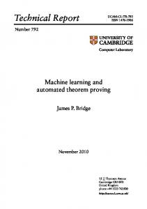
specifies the constraints that the interlocking system must fulfil and is what was verified in this study. More information about the railway domain can be found in (Kerr & Rowbotham 2001, Nock 2002, Leach 2003). The notion of safety used in this study is that trains do not collide and trains do not travel in the facing (diverging) direction over a set of unlocked points; the first conjunct is canonical with respect to loss-of-life and hence safety, whereas the second conjunct ensures that an occupied set of points cannot be moved, hence mitigating a common cause of derailments. To formalise these requirements is was necessary to provide a formal model of a railyard’s topology and a model of the topology’s state. To prove this notion of safety, the signalling principles are specified and proven that they imply the safety of the system. Finally ATP tools are used to provide proofs that the interlocking system fulfils the signalling principles. The interlocking controlled part of Gwili’s topology can be seen in Figure 2, and consists of a number of track segments, signals and sets of points.

Station: Bronwydd Arms 3

16

C2 6

4

C5

1820

19 7

17

Fig. 2. Gwili topology, the dots on the left indicate a single block segment protected by signal 16 (spanning to and including the next stations) that only one train is allowed to occupy at any time. The numbers relate to the controlling leaver, i.e. when leaver 3 has not been pulled, signal 3 shows the danger aspect and when leaver 3 is pulled then signal 3 shows a proceed aspect. The precise differences between the three types of signals (e.g. 3, C5 and 17) is not relevant for this verification and they are treated as main signals. With respect to safety it is clear that signal 4 and 19 should never both be set to proceed as they protect the same part of the track (but in opposite directions), similarly for C5, 7, 18 and 20. Track segments are depicted by horizontal/diagonal lines and delimited by small vertical lines.

Before showing how these topologies are represented, it should be noted that a route with respect to railway signalling can only start at a main signal and ends at the next main signal. Thus each route is in one-to-one correspondence with the signals and spans a number of track segments. E.g. there is a route from signal 3 to signal 4, another from signal 4 to signal C5 and another from signal 17 to signal 16. The topologies are modelled by Segment ∶ Set Train ∶ Set Route ∶ Set

Connected ∶ Route → Route → Set SegInRoute ∶ Segment → Route → Set FacingInRoute ∶ Segment → Route → Set

where axiom Single-Entry-Point is required to hold; it ensures that the routes are well-

Mathematical Structures in Computer Science

21

formed. ∀rt 1 rt 2 rt 3 . Connected rt 1 rt 2 → Connected rt 3 rt 2 → ∃ts . (SegInRoute ts rt 1 ∧ SegInRoute ts rt 3 )

(Single-Entry-Point )

The state of the topology is defined over time, and given as trainRoutet ∶ Train → Route signalAspectt ∶ Route → {proceed, danger} lockedt ∶ Segment → {locked, unlocked} It could be the case that trains ignore the signals and proceed past a danger aspect. As this study was interested in showing correctness of the interlocking system and not obedience of trains to signals, axiom Correct-Trains is required to hold to ensure that trains are well-behaved. ∀t train . (trainRoutet train ≡ trainRoutet+1 train) ∨ (Connected (trainRoutet train) (trainRoutet+1 train) ∧ signalAspectt (trainRoutet+1 train) ≡ proceed)

(Correct-Trains)

To show that an interlocking system is safe, it is required to introduce the following four signalling principles: ∀t route 1 route 2 segment . route 1 ≢ route 2 → SegInRoute segment route 1 ∧ SegInRoute segment route 2 → signalAspectt route 1 ≡ danger ∨ signalAspectt route 2 ≡ danger

(Opposing)

∀t train segment route . SegInRoute segment (trainRoutet train) → SegInRoute segment route → signalAspectt route ≡ danger

(Signals-Guard )

∀t route segment . signalAspectt route ≡ proceed → SegInRoute segment route → FacingInRoute segment route → lockedt segment ≡ locked

(Proceed-Locked )

∀t train segment . SegInRoute segment (trainRoutet train) → lockedt segment ≡ locked → lockedt+1 segment ≡ locked

(Train-Holds-Lock )

The first conjunct of the notion of safety expresses that trains do not collide, and is formalised in Theorem 5.1. It is required initially that all the trains occupy different routes. ∀train 1 train 2 segment . train 1 ≢ train 2 → (Init-Collision-Free) ¬(SegInRoute segment (trainRoute0 train 1 ) ∧ SegInRoute segment (trainRoute0 train 2 )) Theorem 5.1 (Collision Free). Assume axioms Single-Entry-Point , Correct-Trains & Init-

Kanso and Setzer

22

Collision-Free, and that signalling principles Opposing & Signals-Guard hold. Then ∀t train 1 train 2 segment . train 1 ≢ train 2 → ¬(SegInRoute segment (trainRoutet train 1 ) ∧ SegInRoute segment (trainRoutet train 2 )) The proof follows by case distinction on whether train 1 and train 2 have changed routes and from the signalling principles Opposing & Signals-Guard . Signalling principle Opposing expresses that two routes with a common track segment cannot both be set to proceed at the same time. Signalling principle Signals-Guard expresses that any route that has a common track segment with the route a train is currently occupying must show danger aspects. Note that an inexperienced user might overlook the need for the signalling principle Opposing, which is required in order to make sure that two trains don’t enter the same segment. When carrying out a formal proof of Theorem 5.1 the need for such a principle is revealed. This demonstrates that in more complicated real world examples formal proofs using ITP can be crucial to guarantee that the signalling principles are complete in order to guarantee safety. The second conjunct of the notion of safety expresses that trains do not make facing moves over unlocked sets of points, and is formalised in Theorem 5.2. It is required initially that no train occupies an unlocked facing segment. ∀train segment . SegInRoute segment (trainRoute0 train) → FacingInRoute segment (trainRoute0 train) → locked0 segment ≡ locked

(Init-Facing)

Theorem 5.2 (Facing-Point Lock). Assume axioms Correct-Trains & Init-Facing; and that signalling principles Proceed-Locked & Train-Holds-Lock hold, then ∀t train segment . SegInRoute segment (trainRoutet train) → FacingInRoute segment (trainRoutet train) → lockedt segment ≡ locked The proof of Theorem 5.2 is structurally similar to the proof of Theorem 5.1, but instead requires the signalling principles Proceed-Locked & Train-Holds-Lock . Signalling principle Proceed-Locked expresses that when a route shows proceed, then all segments in that route are locked. Signalling principle Train-Holds-Lock expresses that when the segments in an occupied route are locked, then they are locked in the next state. The locking table model of the interlocking system does not have inputs from the trackside equipment; it only consists of a number of leavers that the signalman must pull. It is therefore impossible for the interlocking system to model signalling principles SignalsGuard & Train-Holds-Lock as they require knowledge of the train’s positions. Instead they are enforced by the signalman who observes the railyard and the positions of the trains. In this verification it is assumed that the combination that the leavers are pulled enforce these conditions, i.e. the signalman operates correctly. It should be noted that modern solid-state interlocking systems are provided with train/track detection inputs (as well as many others) so this problem disappears. All that remains is to show that the interlocking system fulfils signalling principles Opposing & Proceed-Locked as they

Mathematical Structures in Computer Science

23

express the conditions under when a route can show the proceed aspect. Due to the finite domains that the topology is built over, it is possible to represent these signalling principles in terms of the output variables of the interlocking, which is then given to a SAT solver to determine un-satisfiablity, after splitting the signalling principles into base and inductive cases. In both cases it was determined that the interlocking system fulfilled the principles. Therefore, by assuming that the signalman does not violate the signalling principles Signals-Guard & Train-Holds-Lock , trains obey signals (axiom CorrectTrains), and showing that the topology fulfils axiom Single-Entry-Point , and showing that the system is initially safe (axioms Init-Collision-Free & Init-Facing), a proof of Theorems 5.1 & 5.2 is obtained, showing that the system is safe. Using the fact that Agda is also a programming language, the locking table was compiled into an interactive program that simulates the interlocking system. It repeatedly requests for the signalman to enter which leaver they wish to move, then executes an iteration of the program and prints out the state of the system. We have successfully applied this technique to a sizable modern interlocking system. It was shown in Agda that the interlocking system fulfilled the signalling principles Opposing, Proceed-Locked , Signals-Guard & Train-Holds-Lock . It still remains to have the model and notion of safety validated. In future work we would like to have validated models. This will require a significant amount of work to formalise the signalling principles and prove that safety follows. This is due to the increased complexities of modern railways. For instance the models would have to consider flank protection and the various systems that ensure trains do not pass signals at danger, or if they do, stop safely. 6. Concluding Remarks This paper explored the differences between interactive and automated theorem proving techniques with a discussion about their respective uses. ATP is used to solve finite concrete theorems and ITP to solve infinite abstract theorems. The discussion was concluded with our motivation for composing these two paradigms, i.e. a proof framework with the advantages of ATP and ITP. We have presented a novel approach to embed an arbitrary ATP theory into type theory, along with two examples of this, namely Boolean tautology checking and CTL model-checking. In its native form, the technique would be very inefficient so we have mitigated this by extending Agda to allow an efficient ATP tool to be called in situ. This has facilitated an efficient framework for proving finite and infinite theorems, specifically with respect to hardware and software verification. The technique described can be used to efficiently define a type, such that elements of this type are correct programs. Such a system would be of use for the development of critical systems as only correct programs can be written, greatly reducing the amount of testing needed. Our vision, which has been partly realised for the train domain, is to use Agda to model domain knowledge; then to develop, verify, compile and execute a substantial program. The motivation here is that a large portion of the software development cycle is contained within a single language and tool; this reduces erroneous translations between languages that occur within typical verification procedures.

Kanso and Setzer

24

We have developed a plug-in mechanism that allows for anybody to embed their chosen ATP theory into Agda by providing the items required in Section 2.2 and Section 3. This plug-in mechanism (modified Agda code), and plug-ins for SAT and CTL can be downloaded from the project website at: http://cs.swansea.ac.uk/~cskarim/agda/ References Abrial, J.R., M. Butler, S. Hallerstede & L. Voisin (2006), ‘An open extensible tool environment for Event-B’, Formal Methods and Software Engineering pp. 588–605. Armand, Micha¨el, Benjamin Gr´egoire, Arnaud Spiwack & Laurent Th´ery (2010), Extending Coq with imperative features and its application to SAT verification, in M.Kaufmann & L.Paulson, eds, ‘Interactive Theorem Proving’, Vol. 6172 of Lecture Notes in Computer Science, Springer Berlin / Heidelberg, pp. 83–98. 10.1007/978-3-642-14052-5 8. Bar-Hillel, Y., M. Perles & E. Shamir (1964), ‘On formal properties of simple phrase structure grammars’, Language and Information: Selected Essays on their Theory and Application pp. 116–150. Barrett, Clark, Roberto Sebastiani, Sanjit A. Seshia & Cesare Tinelli (2009), Satisfiability modulo theories, in A.Biere, M.Heule, H.van Maaren & T.Walsh, eds, ‘Handbook of Satisfiability’, Vol. 185, IOS Press, pp. 737–797. Bierman, G.M., A.D. Gordon, C. Hrit¸cu & D. Langworthy (2010), Semantic subtyping with an SMT solver, in ‘Proceedings of the 15th ACM SIGPLAN international conference on Functional Programming’, ACM, pp. 105–116. B¨ ohme, S. & T. Nipkow (2010), Sledgehammer: Judgement day, in J.Giesl & R.H¨ ahnle, eds, ‘Automated Reasoning’, Vol. 6173, LNCS, pp. 107–121. Boutin, Samuel (1997), Using reflection to build efficient and certified decision procedures, in ‘Theoretical Aspects of Computer Software’, Vol. 1281 of Lecture Notes in Computer Science, Springer, pp. 515–529. Bove, Ana, Peter Dybjer & Ulf Norell (2009), A brief overview of Agda – a functional language with dependent types, in S.Berghofer, T.Nipkow, C.Urban & M.Wenzel, eds, ‘Theorem Proving in Higher Order Logics’, Vol. 5674 of Lecture Notes in Computer Science, Springer Berlin / Heidelberg, pp. 73–78. 10.1007/978-3-642-03359-9 6. Curry, H.B. (1934), ‘Functionality in combinatory logic’, Proceedings of the National Academy of Sciences of the United States of America 20(11), 584. Curry, H.B., R. Feys, W. Craig & W. Craig (1958), Combinatory Logic, Vol. 1, North-Holland. Davis, Martin, Hilary Putnam & Julia Robinson (1961), ‘The decision problem for exponential diophantine equations’, The Annals of Mathematics 74(3), pp. 425–436. de Bruijn, N. (1970), The mathematical language AUTOMATH, its usage, and some of its extensions, in M.Laudet, D.Lacombe, L.Nolin & M.Schtzenberger, eds, ‘Symposium on Automatic Demonstration’, Vol. 125 of Lecture Notes in Mathematics, Springer Berlin / Heidelberg, pp. 29–61. 10.1007/BFb0060623. De Moura, L. & N. Bjørner (2009), ‘Satisfiability modulo theories: An appetizer’, Formal Methods: Foundations and Applications pp. 23–36. Dedekind, R. (1863), Vorlesungen u ¨ber Zahlentheorie, F. Vieweg und Sohn. Diller, J. & A. S. Troelstra (1984), ‘Realizability and intuitionistic logic’, Synthese 60, 253–282. 10.1007/BF00485463.

Mathematical Structures in Computer Science

25

Dong, Yifei, C. R. Ramakrishnan & Scott A. Smolka (2003), ‘Evidence exploration for model checking’. Fontaine, P., J.Y. Marion, S. Merz, L. Nieto & A. Tiu (2006), ‘Expressiveness+ automation+ soundness: Towards combining SMT solvers and interactive proof assistants’, Tools and Algorithms for the Construction and Analysis of Systems pp. 167–181. Foster, Simon & Georg Struth (2011), Integrating an automated theorem prover into Agda, in M.Bobaru, K.Havelund, G.Holzmann & R.Joshi, eds, ‘NASA Formal Methods’, Vol. 6617 of Lecture Notes in Computer Science, Springer Berlin / Heidelberg, pp. 116–130. 10.1007/9783-642-20398-5 10. Harrison, J. (2008), Automated and interactive theorem proving, in O.Grumberg, T.Nipkow & C.Pfaller, eds, ‘Formal Logical Methods for System Security and Correctness’, Vol. 14 of NATO Science for Peace and Security Series, IOS Press, pp. 111–147. Hendriks, D. (2002), ‘Proof reflection in coq’, Journal of Automated Reasoning 29(3), 277–307. Howard, W.A. (1980), ‘The formulae-as-types notion of construction’, To HB Curry: Essays on Combinatory Logic, Lambda Calculus and Formalism 44, 479–490. Huth, M. & M. Ryan (2004), Logic in Computer Science, Cambridge University Press Cambridge. Jones, C.B., G. Grov & A. Bundy (2010), Ideas for a high-level proof strategy language, Technical Report CS-TR-1210, Newcastle University. Kanso, K. (2008), Formal verification of ladder logic, Master’s thesis, Dept. Computer Science, Swansea University. Kanso, K., F. Moller & A. Setzer (2009), ‘Automated verification of signalling principles in railway interlocking systems’, Electronic Notes in Theoretical Computer Science 250(2), 19– 31. Kerr, D. & T. Rowbotham (2001), Introduction to Railway Signalling, Institution of Railway Signal Engineers. Leach, M. (2003), RAILWAY Control Systems, 2nd edn, Institution of Railway Signal Engineers. Lescuyer, St´ephane & Sylvain Conchon (2008), A reflexive formalization of a SAT solver in coq, in ‘TPHOLs 2008: Emerging Trends of the 21st International Conference on Theorem Proving in Higher Order Logics’. M¨ uller, Olaf & Tobias Nipkow (1995), Combining model checking and deduction for i/o- automata, in E.Brinksma, W.Cleaveland, K.Larsen, T.Margaria & B.Steffen, eds, ‘Tools and Algorithms for the Construction and Analysis of Systems’, Vol. 1019 of Lecture Notes in Computer Science, Springer Berlin / Heidelberg, pp. 1–16. Nock, O.S. (2002), Railway Signalling, 2nd edn, Institution of Railway Signal Engineers. Nordstr¨ om, B., K. Petersson & J.M. Smith (1990), Programming in Martin-L¨ of ’s Type Theory, Vol. 7 of International Series of Monographs on Computer Science, Oxford University Press. Owre, S., J. Rushby & N. Shankar (1992), ‘PVS: A prototype verification system’, Automated Deduction CADE-11 pp. 748–752. Paulson, L. & K. Susanto (2007), Source-level proof reconstruction for interactive theorem proving, in K.Schneider & J.Brandt, eds, ‘Theorem Proving in Higher Order Logics’, Vol. 4732, LNCS, pp. 232–245. Stump, Aaron (2009), ‘Proof Checking Technology for Satisfiability Modulo Theories’, Electronic Notes in Theoretical Computer Science 228, 121 – 133. Sutcliffe, G. (2009), ‘The TPTP Problem Library and Associated Infrastructure: The FOF and CNF Parts, v3.5.0’, Journal of Automated Reasoning 43(4), 337–362. Verma, Kumar Neeraj (2000), Reflecting symbolic model checking in coq, Master’s thesis, M´emoire de DEA, DEA Programmation, Paris.

Kanso and Setzer

26

Weber, Tjark (2006), ‘Integrating a SAT Solver with an LCF-style Theorem Prover’, Electronic Notes in Theoretical Computer Science 144(2), 67 – 78. Proceedings of the Third Workshop on Pragmatics of Decision Procedures in Automated Reasoning (PDPAR 2005). Woodbridge, Peter (n.d.), ‘Locking frame testing’. URL: http://www.signalbox.org/branches/pw/index.htm Woodcock, J., P.G. Larsen, J. Bicarregui & J. Fitzgerald (2009), ‘Formal methods: Practice and experience’, ACM Computing Surveys (CSUR) 41(4), 1–36.