A Linear Programming model for the optimal ...

PROCEEDINGS OF ECOS 2012 - THE 25TH INTERNATIONAL CONFERENCE ON EFFICIENCY, COST, OPTIMIZATION, SIMULATION AND ENVIRONMENTAL IMPACT OF ENERGY SYSTEMS JUNE 26-29, 2012, PERUGIA, ITALY

A Linear Programming model for the optimal assessment of Sustainable Energy Action Plans. Gianfranco Rizzoa, Giancarlo Savinob a

Department of Industrial Engineering, University of Salerno,Fisciano (SA), Italy, [email protected] b Energy Manager, City of Salerno, Italy, [email protected]

Abstract: A relevant effort is being spent to reach the EU climate and energy goals by involving European cities and towns in sustainable energy planning. Many Italian and European cities are now involved in the development of Sustainable Energy Action Plans (SEAP), presenting in detailed way the actions finalized to the reduction of CO2 emissions. In most cases, a large number of actions are proposed, ranging from renewable energy production to energy saving and to information and communication actions. It therefore emerges the need of methodologies for guiding the administrators to the selection of the most effective actions for the achievement of the desired emission reduction, compatibly with budget and resource availability. A Linear Programming model for the optimal selection of the actions and of their priorities is presented. The model allows to allocate in optimal way the economic resources among different actions to achieve a given level of CO2 emissions reduction, considering resource constraints. The model has a user-friendly interface, and a complexity compatible with applications to municipal level. An example of application of the model to a school is presented and discussed.

Keywords: Model, Linear Programming, Energy Plan.

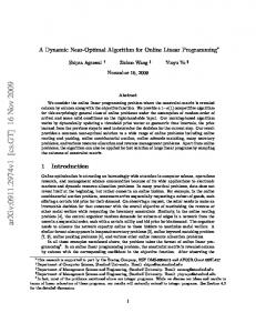
1. Introduction In last decades there are growing concerns about fossil fuel reserve depletion, greenhouse effect and related climate changes. After ratification of the Kyoto protocol [1], a relevant effort is being spent by Europe to enhance renewable energy production and to promote energy efficiency. In December 2008, the EU adopted an integrated energy and climate change policy (20/20/20), with ambitious targets for 2020: cutting greenhouse gases by 20%; reducing energy consumption by 20% through increased energy efficiency; meeting 20% of energy needs from renewable sources [2]. In order to reach these goals, an active participation of European cities and towns in sustainable energy planning has been stimulated by the European institutions. Many European cities are now involved in the development of Sustainable Energy Action Plans (SEAP), presenting in a detailed way the actions finalized to the reduction of CO2 emissions [3]. In Italy, 1225 municipalities have joined the Covenant of Major, while only 16% of them have already produced the SEAP (January 2012) [5]. Most of them are located in the North of Italy (Fig. 1). A study on a set of SEAP produced in eight representative Italian cities (Alessandria, Bergamo, Cesena, Modena, Padova, Piacenza, Torino, Udine) is being carried out by the authors, within the studies to develop the SEAP for the city of Salerno [26] [28]. In most cases, a large number of actions are proposed, ranging from renewable energy production to energy saving, to information and communication actions and to stakeholders involvement. The analysis has demonstrated a certain lack of quantitative data in part of the proposed actions. Moreover, when quantitative evaluations of costs and benefits in terms of CO2 reduction and/or energy savings of each proposed action are provided (Table 1), any indication of priorities or selection criteria among them is missing. Actually, most of the planned actions have quite different cost effectiveness in terms of CO2 reductions and energy savings, as evidenced by the graphs 398-1

reported in Fig. 2, representing: i) the avoided CO2 versus energy savings (upper part) and ii) their unit costs (lower part) for a set of actions and cities (listed in the legend). The analysis of the data shows that there is more than one order of magnitude between the unit costs related to different actions. Moreover, a significant spread between the unit costs of same actions for different cities also occurs [26].

Fig. 1. Number of Italian cities that have completed the SEAP Table 1. Analysis of a group of Italian SEAPs. Actions and Cities. Biomass PV plants LED for traffic lights Street lighting optimization Private Building Optimization Public Building Optimization RSU Thermal Solar Plants District Heating Public Transportation Total

Alessandria Bergamo

1 0 0 0 0 0 0 1 1 1 4

0 1 1 1 1 1 0 0 1 0 6

Cesena Modena

1 1 0 0 1 0 0 1 0 0 4

0 1 1 1 1 0 0 0 0 0 4

Padova Piacenza

0 1 1 1 0 0 0 0 0 1 4

0 0 1 1 0 0 0 0 1 0 3

Torino

Udine

Total

0 0 1 1 1 1 1 1 0 1 7

1 1 1 1 0 1 0 1 1 0 7

3 5 6 6 4 3 1 4 4 3 39

Therefore, it is apparent that a selection criteria between different actions could be needed, at least in case of partial availability of financial resources. Moreover, some of these actions could be mutually exclusive or subject to some common constraints: for instance, space heating requirements could be satisfied by use of solar thermal panels or cogeneration plants, but also reduced by proper building insulation; similarly, the installation of solar thermal panels or photovoltaic panels on building roofs cannot exceed the available surface. It is evident that, in many cases, the decisions about possible alternative actions are somewhat interrelated and not independent of each other. The above considerations evidence the need of methodologies for guiding the administrators to the selection of the most effective actions for the achievement of the desired emission reduction, compatibly with budget and resource availability. A review on the models available in literature for energy and environmental planning is summarized in next chapter, while a model based on Linear Programming, particularly suitable for 398-2

small scale and municipal level, is presented in the following chapters, and some results are discussed. 5

3.5

x 10

3

Avoided CO2 [t*year]

2.5

2

1.5

1

0.5

0 0

1

2

3 4 5 Energy Saving [MWh*year]

6

7 5

x 10

4

2.5

x 10

Avoided CO2 Cost [€/(t*year)]

2

1.5

1

0.5

0 0

500

1000 1500 2000 2500 3000 3500 Energy Saving Cost [€/(MWh*year)]

4000

Modena/PV Bergamo/PV Cesena/PV Udine/PV Padova/PV Torino/Public Transportation Padova/Public Transportation Alessandria/Public Transportation Bergamo/Building optimization (private) Cesena/Building optimization (private) Torino/Building optimization (private) Modena/Building optimization (private) Bergamo/Building optimization (public) Torino/Building optimization (public) Udine/Building optimization (public) Torino/Waste Disposal Bergamo/District Heating Piacenza/District Heating Udine/District Heating Alessandria/District Heating Udine/Thermal solar Alessandria/Thermal solar Cesena/Thermal solar Torino/Thermal solar Cesena/Biomass Udine/Biomass Alessandria/Biomass Torino/LED for traffic lights Modena/LED for traffic lights Piacenza/LED for traffic lights Padova/LED for traffic lights Bergamo/LED for traffic lights Udine/LED for traffic lights Torino/Street lighting optimization Modena/Street lighting optimization Piacenza/Street lighting optimization Padova/Street lighting optimization Bergamo/Street lighting optimization Udine/Street lighting optimization Natural Gas Electrical Energy

4500

Fig. 2. Analysis of a group of Italian SEAPs. Avoided CO2 vs Energy savings (up) - Avoided CO2 Unit Cost vs Energy savings unit cost (down)

398-3

2. Models for Energy Systems Several models have been developed to study and plan the evolution of complex systems involving interaction of economic, energetic and environmental aspects. A large review of models used for energy studies, at different levels and approaches, is available in [20]. In the early ‘70s, the model WORLD3 was used to model the interactions between population, industrial growth, food production and limits in the ecosystems of the Earth [6]. Some years later, the MARKAL models generator was developed by a consortium of 14 countries under the aegis of an IEA committee (Energy Technology Systems Analysis Development Programme, ETSAP), with a specific focus on energy system analysis [7]. Starting from the original formulation, further implementations have been carried out to account for different situation and purposes. A short overview of MARKAL models is presented in Table 2. The mathematical approach is mainly based on Linear Programming (LP), while Non-Linear Programming (NLP), Multiple Integer Programming (MIP) and Stochastic Programming (SP) are also used. Further details, with reference to selected bibliography, is available in [8]. The MARKAL models are now widely used in many countries to support energy-environmental planning at national and local scale [9][10][11]. Specific tools have also been developed at the Environmental Protection Agency (EPA) in U.S.. The “Integrated Planning Model” (IPM) allows to analyze the impact of air emissions policies on the U.S. electric power sector. EPA has used multiple iterations of the IPM model in various analyses of regulations and legislative proposals [13]. Table 2. Overview of the MARKAL family of models (from[8] ). Member /Version

Type of Model

MARKAL MARKAL-MACRO

LP NLP

MARKAL-MICRO

NLP

MARKAL-ED (MED)

LP

MARKAL

NLP

MARKAL

LP

MARKAL

SP

MARKAL – ETL

MIP

Short Description Standard model. Exogenous energy demand Coupling to macro-economic model energy demand endogenous. Coupling to micro-economic model, energy demand endogenous, responsive to price changes. As MARKAL-MICRO but with step-wise linear representation of demand function. Linkage of multiple countries specific MARKAL-MED With multiple regions and MARKAL-MACRO, including trade of emission Permits. Besides energy flows (electricity, heat) material flows with material flows and recycling of materials can be modeled in the RES. Stochastic Programming. Only with standard model. With Uncertainties Endogenous technology learning based on learning-by-doing curve. Specific cost decreases as function of cumulative experience.

Some models address specifically the energy plans at municipal level [21]-[25]. Both general models [21] [22] [25] and specific models, i.e. for Solid Waste Management [23], have been developed. However, in some cases the term ‘municipal’ may be misleading, being referred to very large communities as Beijing [21]. The MARKAL and IPM models, in their numerous versions, can cover most, if not all, of the possible cases occurring in the study of an energy and environmental system, and could certainly be adapted to study actions at municipality level, as considered by SEAP. However, their modelling structure is quite complex, and their use is probably more suitable in academic and government agencies context rather than at municipal level, in particular for a small or medium size town or city. On the other hand, at a local level interactions with macro-economic aspects, material flows 398-4

and prices changes, representing the distinctive features of the MARKAL or IPM models, are of course less relevant than at regional or national level. In next chapter a simpler LP model will be presented, specifically tailored to the exigencies of small scale systems, as for a SEAP at municipal level.

3. The proposed LP model The proposed methodology is based on the solution of an optimal resource allocation problem by means of a Linear Programming (LP) approach. The classical LP problem consists of the determination of the decision variable vector x minimizing a linear objective function F(x): ∗

(1)

(2)

subject to linear equality constraints: ,

and to linear inequality constraints: (3)

Starting from its basic formulation from Dantzig [15], several different versions of LP methods have been proposed, for the solution of different problems. In the present case, the solution is obtained by means of the Simplex method, as implemented in the Matlab function ‘linprog’ [16]. The decisions variables xi represent a measure of the investment in each action. Their units vary according to the specific action considered, as specified in Table 3. Regarding their nature, xi are real and non-negative numbers. In case of LED, x3 should be indeed an integer number, representing the optimal number of lamps. However, it is treated as a real number, being its value quite large (particularly in applications at municipal level). The result of the optimization problem is therefore approximated to the nearest integer number. The objective function F(x) (1) is expressed as a linear combination of the product of decision variables xi and terms fi: (4)

where ii is the yearly unit investment and ri is the yearly unit revenue associated to the i-th action, while T is the time horizon, in years. The objective function therefore represents the global investment needed by the decision maker (the municipality) to achieve a given level of CO2 emissions, minus the possible revenues associated to the actions, achieved in the given time horizon. Both short and long terms strategies can be examined by varying T. In particular, if T is set to zero, no revenues are considered. Therefore, the solutions corresponding to the minimum investment needed to achieve the given level of CO2 reduction are sought. This solution would then represent the minimum cost strategy to achieve the given emissions reduction, regardless of future revenues. The variable Beq in the equality constraint (2) represents the global reduction of CO2 emission, while the diagonal terms of the matrix Aeq contain the unit impact factors of the actions xi on CO2 emissions. The inequality constraints (3) express the availability of resources to be allocated to the actions x, where variable B is the maximum available resource for each group of actions, and the matrix A indicates the correspondence between each action and a group of resources. An additional inequality constraint (5) expresses the conditions that the total required investment I must be not greater than the available economic resource Imax:

398-5

(5)

The solution of the problem is achieved for two scenario’s with different time horizon, i.e. Short Term (T=0) and Long Term (T=20). In the former case, the solutions corresponding to the minimum investment compatible with the given emission reduction are obtained, regardless the long term result. In the second case, the maximum long term results are obtained, of course with a greater initial investment. The results corresponding to intermediate investment values between these two limit cases are also investigated, by imposing suitable values to the maximum allowed investment in (5). For each scenario, the whole range of emissions reduction Beq is examined. Therefore, a complete picture of the required actions, of their priorities and of the needed investment is provided, both in tabular and in graphical form. Some general comments on the linear assumption of the model seem necessary. As shown in Table 2 and in literature review presented in the previous chapter, Linear Programming is one of the most used techniques for energy planning problems. Although most physical systems involved in such problems are inherently non-linear in nature, the relationship between the decision variables and the output variables can often be approximated by linear relationships. With reference to the actions considered in this paper and in the on-going applications to municipal level, there are certainly some scale effects related to the size of the plant, affecting unit costs, and possibly efficiencies and CO2 emissions. In case that these effects are relevant, they could be treated by non-linear relationships, so leading to a non-linear optimization problem, characterized by a significant increase in complexity and computational burden with respect to a LP problem. Another way to tackle the problem is to consider separately the actions referring to small, medium or large plants, where each class of plants can be characterized by (approximate) linear relationships between decision variables and output variables. This approach, that seems more suitable at small or medium scale energy systems, could allow to maintain the advantages of Linear Programming with only a moderate increase in problem dimensionality.

4. An example of application In order to check the operation of the model on a small scale example, the case of a school has been considered. The energy required is for space heating (in the period from November 15 to April 30) and electricity and hot water (all the year, except August), while no air conditioning is required. Different solutions have been considered: A. Solar thermal collectors for hot water and space heating, with seasonal storage. B. Photovoltaic (PV) panels (the surplus electricity is sold to the grid). C. Reduction of electricity demand by adopting LED. D. Cogeneration plant (CHP), fueled with natural gas (the surplus electricity is sold to the grid). E. Reduction of thermal energy demand by building insulation. Investment costs, yearly savings and avoided CO2 per unit are reported in Table 3, for each action. They represent respectively the terms i and r in equations (4) and (5), and the terms Aeq in equation (2). For instance, in case of PV panels (second row) the decision variable x2 is represented by panel surface in m2, the term f2 (4) is equal to 300-50·T, while 70 is the estimated yearly avoided CO2 per unit (square meter), representing the term Aeq2,2 in the equality constraint (2).

398-6

Table 3. Actions, unit cost, savings and avoided CO2. Unit Actions Thermal Solar + Seasonal Storage PV panels LED CHP with methane Building insulation

m2 m2 No. of lamps kWe €

Unit cost € 750 300 100 2000 1

Savings €/year/unit 50 40 20 680 0,24

Avoided CO2 kg/year*unit 300 70 50 1600 0,45

The links between actions and resources are summarized in Table 4. In the second row the maximum available resource for each action is reported, representing the terms B in equation (3). They express the maximum allowed surface for solar panels (the sum of thermal and photovoltaic), the maximum number of LED lamps, the maximum electric power for co-generator and the actual thermal load of the building. The correspondence between each action and the resources, representing matrix A in (3), is also presented in the lower part of the table. In this case, the matrix expresses a link between solar thermal panels and PV panels (second column), whose surface cannot exceed the total available surface of 200 m2. A further constraint (last column) connects thermal panels, CHP plant and building insulation, since their effect cannot exceed the given yearly thermal load, estimated in 91500 kWh. In other words, their effects are additive, and should not exceed the required thermal load to avoid energy waste. The use of LED lamps, instead, is not linked to the other actions related to electrical energy production (PV panels and CHP), since it is assumed that the excess electrical energy can be sold to the grid. Table 4. Actions and available resources. Resource Availability Actions Thermal Solar + Seasonal Storage PV panels LED CHP with methane Building insulation

Panel Surface [m2] 200

N lamps [/] 80

CHP [kWe] 100

Thermal load [kWht/year] 91500

1 1 0 0 0

0 0 1 0 0

0 0 0 1 0

450 0 0 17520 2,25

The data in the tables have been estimated starting from average producibility of solar plant, cost of natural gas and of electricity in Italy, studies on thermal solar plants with seasonal storage and literature data on building insulation costs and performance. It has to be remarked, however, that the main purpose of this calculation is to check and illustrate the features of the proposed method, rather than to design in detailed way the best energy system for a school. Of course, more precise and complex methods exist for thermal design and optimization of buildings, also including nonlinear and transient effects, that are not considered in this analysis [17], [18], [19].

4.1. Results A global picture of the results, in terms of investment, costs and CO2 reduction, is provided in Fig. 3. The optimal size of investment and the related profit for each action is shown in Fig. 4, for the two scenarios (short term and long term). It is timely to remark that, both in short and long term scenarios, profits are evaluated after the same time horizon (i.e.20 years). However, while in long term scenario profit coincides with the objective function (1), in the short term case (T=0) the long term profit corresponding to the minimum investment is computed. 398-7

Cost-Benefit - Short Term vs Long Term Strategies 0.35 Investment (st) Profit (st) Investment (lt) Profit (lt)

0.3

0.25

M€

0.2

0.15

0.1

0.05

0 10

20

30

40

50 60 70 CO2 Reduction [%]

80

90

100

Fig. 3. Optimal results - Investment Costs and Profit vs CO2 reduction In Fig. 3, the short term scenario is indicated by continuous lines, while dotted lines represent the long term scenario. To achieve a given CO2 reduction, different solutions are available, with investment costs ranging from a minimum value (continuous blue line) to a maximum value (dotted blue line). In correspondence, profit also ranges from a minimum value (red continuous line) to a maximum value (red dotted line). Intermediate results are indicated by blue and red stars. It can be observed that the investment costs (blue lines) are always increasing with CO2 reduction. The dotted line stops at 0.1 M€, representing the maximum allowed investment Imax. The slope of profit (red lines), instead, tends to decrease, and to become negative. This tendency is much more evident for the dotted line (long term). In this case (upper part of Fig. 4), the actions corresponding to higher profit per avoided emission unit are first selected (building insulation, in this case), then the other actions (PV panels, LED and thermal panels). It can be observed that, when the emission reduction increases, a gradual substitution between PV and thermal panels occurs, due to the constraint on maximum available surface. Similarly, the investment in building insulation decreases when thermal solar panels are adopted. For the actions not conflicting with others (i.e. LED lamps), the investment gradually increases until the saturation level is reached. For the short term scenario (lower part of Fig. 4) the most convenient solutions in terms of initial investment versus CO2 reduction are first selected. In this case, the suggested actions are CHP, LED and thermal solar panels. It can be also observed that, when investment for thermal solar panel increases, the size of CHP plant is reduced, to satisfy the constraint on the thermal load. It can be observed that there is a large difference between the minimum and the maximum profit, corresponding to short and long term scenarios. The difference is small at lower investment values, growths to their maximum at about 87% of CO2 reduction, when the maximum allowed investment (blue dotted line) reaches the limit value of 0.1 M€ (Fig. 3). After this value, the differences between short and long terms scenarios tend to decrease again. It emerges, therefore, that, for a large range of CO2 emissions, even small differences in investment costs (blue) may produce large differences in profit, at the same level of CO2 emissions. An analysis limited only to investment costs and related CO2 emissions could therefore strongly penalize the long term results, while much better profits could be obtained with only a slight increase in initial investment. 398-8

Time Horizon=20[year]


0.06

0.2 0.15

0.04

Profit [M€]

Investment [M€]

0.05

0.03 0.02

0.1 0.05

0.01 0 0

50 CO2 Reduction [%]

0 0

100

Time Horizon=0[year] 0.08

0.08

0.06 Profit [M€]

Investment [M€]

100


0.1

0.06 0.04

0.04 0.02

0.02 0 0



0 0

100


100

Thermal Solar + Seasonal Storage PV with incentives LED CHP with methane Building insulation

Fig. 4. Optimal results - Investment and profit for each action vs CO2 reduction It is worth noting that the CO2 reduction can even exceed 100% of the original CO2 emissions. In fact, the production of electrical energy via CHP and PV panels is not necessarily limited to the electrical load of the school, since it can be sold to the grid. A graph with the ratio between profit and investment is presented in Fig. 5. This ratio ranges between 1 and 5,5, approximately. Similar graphs are obtained to describe the optimal size of the proposed actions, versus CO2 reduction and investment. Two graphs refer to optimal surface of PV plant, reaching their maximum value at a CO2 reduction of about 75% (Fig. 6), and to optimal number of LED lamps, that tend to be selected only for CO2 reduction greater than 30% (Fig. 7). Similar graphs, not reported in the paper due to space constraints, are obtained for the other planned actions. The set of results presented above has been obtained by solving the LP problem (1)-(5) 45 times, for different values of constraints on CO2 level and maximum allowed investment. About 100 graphs and several tables in Excel were automatically generated. Computational time is about 50 seconds on a Desktop PC (CPU Intel® Core™ i3, 4 GB RAM, 3.07 GHz). These results demonstrate that, even considering a relatively simple energy system as a school, a rather complex picture emerges and articulate strategies are needed to achieve the best results in 398-9

terms of CO2 reduction, with limited economic resources and in presence of constraints between the different actions. The best mix of solutions depends on the target emission reduction, and therefore on the available financial resources. Moreover, even if provided by a linear model, the solutions are not linear with respect to the output (CO2 emissions reduction): in other words, the best solution to achieve 100% reduction of CO2 is not simply obtainable (i.e. doubling each action) from the solution corresponding to 50% reduction, as clearly shown in Fig. 4. In fact, passing from 50% to 100% reduction, the best solution is obtained not only incrementing some actions, but also reducing some others. This implies that a clear picture of objectives and of available resources is required at the start of the project, since the best strategy to enhance system performance (i.e. increase CO2 reduction) could not be simply obtained by additional investments on an existing plant, even if starting from an optimal solution. Profit/Investment

Investment [M€]

0.1

5.5

0.09

5

0.08

4.5

0.07

4

0.06

3.5

0.05

3

0.04

2.5

0.03

2

0.02

1.5

0.01

1 20

30

40


80

90

100

Fig. 5. Optimal results – Ratio between profit and investment vs. CO2 reduction. PV with incentives 0.1

160

0.09

140

0.08 120 Investment [M€]

0.07 100 0.06 80

0.05 0.04

60

0.03

40

0.02

20

0.01 20

30

40


80

90

100

Fig. 6. Optimal results – Optimal surface of PV panels (m2) vs. CO2 reduction.

398-10

LED 0.1

80

0.09

70

0.08 60 Investment [M€]

0.07 50 0.06 40

0.05 0.04

30

0.03

20

0.02

10

0.01 20

30

40


80

90

100

Fig. 7. Optimal results – Number of LED lamps vs. CO2 reduction.

5. Conclusions A methodology to assess the optimal combination of actions to achieve given CO2 emission reduction, considering their effectiveness and costs, has been presented. The proposed procedure is particularly suitable at a municipality level, to assist the development of Sustainable Energy Action Plans. The methodology, based on a Linear Programming approach, provides the optimal selection of the actions and of their priorities in order to achieve the best environmental benefits in presence of limited economic resources and of constraints between the different actions. The results, obtained by application of the model to a school, have evidenced that not straightforward strategies can be required to achieve the best mix of the planned actions in order to maximize the environmental benefits, for different availability of economic resources. It has also been shown that the analysis cannot be limited to the minimization of investment costs for given emission reduction, since long term effects could be significantly penalized by this approach. This result is of practical relevance for the assessment of the Sustainable Energy Action Plans, since in most of the analyzed cases only investment costs and impact on CO2 emissions were provided in the documents, regardless of their long term economic impact. This approach could lead into significant inefficiencies in terms of allocation of financial resources. The procedure is actually in course of application to the development of Sustainable Energy Action Plan for the city of Salerno, in South Italy. In this case, the actions are being treated at aggregate levels (i.e. buildings are not described individually, but as clusters of homogeneous cases; the same happens for infrastructures and transport systems). A study on SEAP of different Italian cities [5] [26] [28] has shown that the number of different actions considered is of the order of ten (Table 1). It is therefore expected that the total number of actions will be not very large, and that it will compatible with the proposed method, in terms of computational burden and of robustness.

References [1] The Kyoto Protocol, available at [2] European Commission, Climate Action Documents and Publications, available at [3] P.Bertoldi, D.Bornás Cayuela, S.Monni, R.Piers de Raveschoot, Existing Methodologies and Tools for the Development and Implementation of Sustainable Energy Action Plans (SEAP), 398-11

Publications Office of the European Union, 2010, JRC56513, ISBN: 978-92-79-14852-1, ISSN: 1018-5593. [4] Convenant of Majors, available at [5] Italian Cities belonging to Convenant of Majors, available at [6] D.H. Meadows, D.L. Meadows, J.Randers, and W.W. Behrens III. (1972), The Limits to Growth. New York: Universe Books. ISBN 0-87663-165-0. [7] Fishbone LG, Abilock H., MARKAL - A linear-programming model for energy system analysis: technical description of the BNL version. Int J Energy Res 1981;5:353–75. [8] Mohammad Reza Faraji Zonooz, Z.M. Nopiah, Ahmad Mohd Yusof, Kamaruzzaman Sopian, “A Review of MARKAL Energy Modeling”, European Journal of Scientific Research, ISSN 1450-216X Vol.26 No.3 (2009), pp.352-361 [9] E. Endoa, M. Ichinoheb, Analysis on market deployment of photovoltaics in Japan by using energy system model MARKAL, Solar Energy Materials & Solar Cells 90 (2006) 3061–3067 [10] M. Salvia, C. Cosmi, M. Macchiato, L. Mangiamele, Waste management system optimisation for Southern Italy with MARKAL model, Resources, Conservation and Recycling, 34 (2002) 91–106. [11] Johnsson J, Bjorkqvist O, Wene C-O. Integrated energy-emissions control planning in the community of Uppsala. Int J Energy Res 1992;16:173–95. [12] ETSAP, Energy Technology Systems Analysis Program, available at [13] EPA Integrated Planning Model, available at [14] City Energy Plan, Salerno (in Italian), available at [15] G.B Dantzig, Maximization of a linear function of variables subject to linear inequalities, 1947. Published pp. 339–347 in T.C. Koopmans (ed.):Activity Analysis of Production and Allocation, New York-London 1951 (Wiley & Chapman-Hall). [16] Linear Programming on Matlab, available at [17] D.B. Crawley, L.K. Lawrie, F.C. Winkelmann, W.F. Buhl, Y.J. Huang, C.O. Pedersen, R.K. Strand, R.J. Liesen, D.E. Fisher, M.J. Witte, J. Glazer, EnergyPlus: creating a new-generation building energy simulation program, Energy and Buildings, pp. 319-331, vol. 33, 2001 [18] J. A. Clarke, J. Cockroft, S. Conner, J. W. Hand, N. J. Kelly, R. Moore, T. O'Brien, P. Strachan, Simulation-assisted control in building energy management systems, Energy and Buildings, pp. 933-940, vol. 34, 2002. [19] Building Energy Software Tools Directory, US Dept. Of Energy, available on http://apps1.eere.energy.gov/buildings/tools_directory/subjects_sub.cfm [20] S. Jebaraja, S. Iniyanb, A review of energy models, Renewable and Sustainable Energy Reviews, 10 (2006) 281–311 [21] Q.G. Lin, G.H. Huang, Planning of energy system management and GHG emission control in the Municipality of Beijing - An inexact-dynamic stochastic programming model, Energy Policy 37(2009) 4463–4473. [22] Clas-Otto Wene, Bo Rydén, A comprehensive energy model in the municipal energy planning process, European Journal of Operational Research, Volume 33, Issue 2, January 1988, Pages 212–222

398-12

[23] Guohe Huang, Brian W. Baetz and Gilles G. Patry, A Grey Linear Programming Approach for Municipal Solid Waste Management Planning under Uncertainty, Civil Engineering Systems, Volume 9, Issue 4, 1992 [24] Jenny Ivner, Municipal Energy Planning – Scope and Method Development, PhD Thesis, Linköping Studies in Science and Technology, Dissertation no. 1234 [25] Dag Henning, MODEST—An energy-system optimisation model applicable to local utilities and countries, Energy, Volume 22, Issue 12, December 1997, Pages 1135–1150 [26] Daniele Galdi, Piani d’Azione per l’Energia Sostenibile: analisi quantitativa delle azioni proposte, Bachelor Thesis in Mechanical Engineering, University of Salerno, February 2012, in Italian. [27] Gabriele Orlando, Modelli per la pianificazione energetica ed ambientale, Bachelor Thesis in Mechanical Engineering, University of Salerno, February 2012, in Italian. [28] Vito Di Guida, Analisi comparata dei Piani d’Azione per l’Energia Sostenibile, Bachelor Thesis in Mechanical Engineering, University of Salerno, February 2012, in Italian.

Acknowledgments The contributions given to the present analysis by Vito Di Guida, Daniele Galdi and Gabriele Orlando during their Master Thesis in Mechanical Engineering at the University of Salerno are gratefully acknowledged.

398-13