A Localisation Method with an Omnidirectional

Proceedings of the 1998 IEEEJRSJ Inti. Conference on Intelligent Robots and Systems Victoria, B.C., Canada October 1998

A Localisation Method with an Omnidirectional Vision Sensor Using Projective Invariant Bruno MARHIC, El Mustapha MOUADDIB' IEEE member, and Claude PEGARD. Universite Picardie Jules Verne (UPJV) Groupe de Recherche sur l'halyse et la Commande des SYst6mes (GRACSY) 7 rue du MOULIN NEW, 80 000 AMIENS, France E-mail: [email protected]

Abstract In this paper, we first present a short description of our conic sensor. Furthermore, we will pay special attention to the famous projective invariant, represented by the cross-ratio. We will end this paper by presenting a new ID cross-ratio application that enables us to localise our mobile robot SARAH efficiently. With the method that we propose using, the camera does not need to be calibrated and this vision system, based on an omnidirectional sensor, is a major advantage for the navigation of an autonomous mobile robot.

1

Introduction

The principal task of computer vision is object or scene recognition. In most vision-based approaches for localisation, environment modelling is rendered complex as the geometric properties are not invariant to the projective transformation nor to the change of viewpoint [SI. Moreover, the matching phase is generally very complex and time consuming and most approaches require camera calibration. Our previous dealings with an omnidirectional vision system are exposed in [13][14]. In [13], the approach is purely combinational and is not completely immune to the parasite straight lines of the image. We define parasite straight lines as all straight lines that do not correspond, a priori, to a recorded reference point on the map. In [ 141, a solution to the problem of parasite straight lines is suggested by fusing the odometric sensors with the omnidirectional vision. The method suggested in [I41 renders good results, but does necessitate a fusion of the sensors. hi a recent work [15], K.S. Roh et a1 use projective invariants to localise a mobile robot. However, their method requires a vanishing point formed by the image of a corridor in order to be able to calculate an invariant in the scene. In this paper, we present a new application of 1D cross-ratio (and its dual for four lines), in order to resolve the matching between the model (in any type of environment) and an omnidirectional image of the scene. Our matching method is trivial and does not require +

camera calibration as we also use geometric projective invariants [Ill. What are invariants? The idea of invariance in computer vision appears when one has analysed the human ability to recognise objects. Invariants are quantities that allow for matching an object (or a scene) in an image with a model, no matter the transformation applied to the model and no matter the viewpoint. We use the term "transformation" in its larger sense, meaning that it can contain the composition of several elementary linear transformations (rotation, translation, scaling, shearing...). More the transformation is general, complex, more it is difficult to find invariants. This leads us to the unavoidable question: for which type of geometric transformation do we want to calculate an invariant quantity? The major part of invariants listed in the computer vision literature are intrinsic invariants, more often called geometric descriptors or geometric invariants ; however there are also non-geometric invariants called extrinsic invariants [2]. We can distinguish two significant classes of invariants: global invariants (or integrals) [3] and local invariants (or dzfferentials) [4]. A global invariant defines information on the object in its entirety, which renders it quite insensitive to noise. Such invariants necessitate knowledge of the entire object or scene, but are rather sensitive to occlusions. A local invariant defines information on a point or a small unity of points (semilocal) independently of the other points that constitute the contour of the object. These invariants (local and semilocal) are much more immunised to occlusions as the contour is not used in its entirety, but are rather sensitive to noises, which implies that in most cases a preliminaiy image filtering is needed. Generally, differential invariants methods require high orders of derivatives for calculating invariants, which is not without consequences for the reliability of these methods. Eventhough all invariant quantities can normally be classed in either the globallintegral invariant family, or in the localldifferential invariant family, the algebraic invariants merit a new class. Algebraic methods imply the calculation of implicit polynomes of the contour [ 5 ] , such

PhD Tutor of B.Marhic.

0-7803-4465-0198$10.00 0 1998 IEEE

1078

as conics, quadrics, etc. Therefore, contrary to differential invariants that are defined locally (a point), algebraic invariants remain constant for the entire implicit polynome considered; algebraic invariants are regional invariants (between local and global) and are much less sensitive to image noises compared to differential invariants. Examples of algebraic invariants are given in [61. Using quasi-invariants, that are easier to obtain than invariants, might prove helpful. Unfortunately, these quantities (quasi-invariant) are only "invariant" on the limited transformation range for which they were calculated.

2, the line L' in the image plane (n) is the projective line of L with point 0 as the centre of projection; this geometric transformation i:j the fundamental 1D projective transformation. The 1D projective mapping between lines is given by the 2x2 homogtmeous transformation matrix T, so that x = T.X where [x,:,x2ITare the homogeneous coordinates on the transformed line. There are three essential parameters to defiie the matrix T (over scale of T is not important).

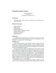
Intrinsic properties of our conic 2 sensor: SYCLOP' Our conic sensor is made up of two essential parts: a CCD camera and a conic reflector (Figure 1-a). These two parts are separated by a glass support. This type of perception system is also used by YAGI [l] with the COPIS system. An example of an image generated by the omnidirectional sensor is given in Figure 1-b.

- -(a) (b) Figure 1: The omnidirectional sensor and a conic image. Advantage for navigation: Associating a conic mirror with a camera enables us to obtain a panoramic image (360O) of the robot's environment. This characteristic is a major asset to the navigation of an autonomous mobile robot, as it takes away the robot's "direction of the vision field" constraint for a given robot's configuration XT=[xr, yr, Or]lRc, where Re is the absolute reference of the environment. This property of omnidirectionality offers a better chance for the matching phase between models and the scene and, therefore, a higher chance of localising itself according to the landmarks of the environment. Geometrical advantage: The use of this particular sensor enables us to modelise the 3B environment of the robot into a simple 2D map, containing reference points expressed in the fiame Re. These points represent the vertical landmarks of the environment. The orthographic projection of the vertex S of the cone (which lies on the revolution axis A), gives the point 0 in the image plane ( x ) . This point 0 is materialised through the intersection of the virtual view lines in the image. Therefore, this point 0 is a virtual projection centre. As we can see from Figure

Figure 2: Radial straight lines formation and the 1D projective transformation.

3

Theoretical Preliminaries

3.1

Basic theory of cross-ratio

Cross-ratio (also lcnowni as anharmonic-ratio) has been recognised for a long time as being the most fundamental projective invariant. All other projective invariants can be derived fiom the cross-ratio. We would like to give one historical example. In 1827, the mathematician AF Misbius [7] proved the invariance of 1D cross-ratio and these generalisations to triangle areas and tetrahedric volumes. Chapter 11 of [SI presents, in a clear and relatively concise fashion, the cross-ratio for its use in computer vision. Let PI,..,4 be any four collinear points in the plane. The following theorem [9], defines the cross-ratio: Theorem: The cross-rutio of distances between any four points in the object h e is the same as the cross-ratio of distances between their images in any image line (Figure 3).

Let p be the cross-ratio of the 4 collinear points:

where DGis the distance from Pi = [xi, yiIT to P, = [x,, y,IT along the line L (idem for Dij). The cross-ratio is an absolute invariant. Proof of the preceding theorem is given in [9].

~~

' SYstkme conique pour la Localisation et la Perception. 1079

(P'-P+f I3(P) =

(4)

P2(P-1)'

Figure 3: Theorem for point projections and cross-ratios. Fundamental theorem preserves the cross-ratio.

[111:

Any

homography

A homographic transformation is any linear transformation in homogeneous co-ordinates, including central projection (perspective projection), linear scalings, skewings, rotations, translations ...Thus,our conic sensor preserves the cross-ratio. Since points and lines are dual, an equivalent crossratio for lines exists. The dual relation to collinearity is incidence at a point. A cross-ratio is defined on four lines which are incident at a single point. Any set of lines incident at a common point is called a pencil. The crossratio of a pencil can be defined in terms of the angles between the lines as shown in Figure 4, and is given by:

where I&) is called the j-invariant. Unfortunately, the use of such functions (I1 and 12) of p is very dainty as these functions are unstable. As a matter of fact, only one crossratio needs to be unstable to render the functions IklJ(p) unstable as well. The use of the j-invariant (eq. (4)) is preferable.

3.2

Calculation of the Position

In the static case, the robot's configuration is given by the vector X:

where (G ,yc) are the robot's co-ordinates in the world frame Re and 8 is the robot's orientation in the same frame. The robot's configuration is determined by the equations linking the sensorial radial straight lines (in the image) with the co-ordinates of the landmarks (eq. (5)). Yc-Yi

tan(6 + + i ) = ~, xc -xi

(1bis)

where is the relative angle of the landmark Bi in the robot's frame Rr and (xl ,yi) are the co-ordinates of the landmark Bi. We obtain one equation for each matched radial straight line. The system of non-linear equation obtained is identical to the one managed by the goniometrical localisation methods [ 161. We refer the interested readers to [ 13][ 141, where this localisation method is treated.

4 Figure 4:The dual configuration for the cross-ratio. Unfortunately, the cross-ratio depends on the order in which the points are marked. If the labels of the four points are permuted, the cross-ratio of four points renders only six different values (of which three are the inverse of the other three) for twenty-four (4!) possible labelisations. The six different values in relation to p are [lo]: P1= P

P3=1 - P

P5 = P1(-P*)

P2 = P i 1

p4 = p3-'

P6 = PZ(-P3)

On the basis of the discussion above, our experimental results with real images are shown. We have implemented our localisation algorithm on the mobile robot SARAH. The map of the environment is known a priori. The environment's map creation is an off-line process. This map is simply a set of reference points in the world's reference frame Re. These points represent the absolute location of the vertical landmarks (doors, wall's junctions...).

4.1 In order to remedy this numeration problem (that can hinder the recognition of objects), we can use symmetric functions of p, that are invariant to the permutation of labels [11][12]. The functions Il(p), I&), and 13(p) are examples of permutation invariant functions: Il(p)

=

ci=1 ,...

6 Pi 9

Experimental Results

Candidates' formation for matching

In order to simplify the following experimental results, we voluntarily limited ourselves to determining just one invariant-model with two aligned and contiguous doors of our laboratory (Figure 5). It is easy to generalise the following principle €or each quadruplet of collinear points of the environment's map and design a model table.

(2) 1080

Invariant-model design: As we mentioned above, we calculate an invariant-model pair with two doors. We simply apply the equations (1) and (4), where D13= dist(P1,P3) = 117.7 Cm, DL4= 198 Cm, DZ4= 107.5 Cm et Dz3= 27.2 Cm. The value of the model-invariant is given by the (pmod, jmd) pair (eq. (6)). The evaluation of the model-invariant is an off-line calculation.

i

Pmod = (1 17.7 /

198) / (27.2 / 107.5) = 23494

(6)

jmod= 7.2161

1)

Rejection criteria

I

NbofCandidates (a) (b) (c) (d) 7315 3060 7315 7315 2114 1115 1381 2225

I

1 d(pmod,pi)'0.006

Primitive extraction: For each image, we first apply a low pass filter of a 3x3 weighted kernel window in order to reduce the noise. We then calculate a 3x3 Sobel filter in order to extract the boundaries of the conic image (Figure 6). Finally, we apply a modified Hough transformation in order to design the conic image's radial straight lines (Figure 7). Candidates formation: Let n be the number of primitives extracted from the conic image. Then, there are C(n,4) combinations of quadruplets of straight lines. We calculate one cross-ratio for each quadruplet and compare it with the model. As the cross-ratio is not a metric dimension, a comparison by difference makes no sense. We have to implement the distribution function F(p) of the cross-ratio to be able to compare the different crossratios. Thus, we take the following equation [I71 as the distance between two cross-ratios: d(P,,P2) = min(lF(p1) - F(P2 $1 - IF(P1) - F(P2

notice that invariants (pmo,d,jmd) are between mp,j f op,j ; this shows that ID cross-ratio is reliable, when one considers projective transformation.

I

I

I

~

175 63 58 105 Table 1: Number of candidates &er the different criteria.

I

I

Crow Ratio

I

J-invariant

I 1 1

Y

where F is the distribution function. The projective distance d will ly between 0 and %. Then, we reject all cross-ratios too far &om the model. We also apply two trivial criteria to decrease the number of candidates. First, as the model is calculated &om four aligned points on the same wall, we can reject, without any loss of information, the angular sectors (formed by the lines of the quadruplet) bigger than 180 degrees. Secondly, we can also reject all the angular sectors smaller than 10 degrees, this means that the robot is too far f2om the four landmarks. All the non-rejected quadruplets are candidates for the matching\localisation step. The following table, the Table 1, shows the effects of the different criteria on the numbers of candidates for the images (a)...(d) of the Figure 7. Table 2 shows the values of invariants for the quadruplet of straight lines in the image that correspond with the vertical landmarks that have served to determine the model-invariant. There is an invariant pair for each image (a), ...(d) of Figure 6. In Table 2, we have also shown the mean m over the four images, the standard deviation Q and the percentage of the standard deviation to the mean. Table 2 shows that, essentially, all of the values pi and ji are constants; they remain stable in spite of the change in viewpoint. This shows that the values of the invariant are reliable, even for noisy images. One can also

Figure 5 : Geometric configuration for the model.

4.2

Matching and lalcalisation

The use of invariants makes the matching phase trivial and efficient. We calculate a hypothetic configuration for each selected quadruplet in the image. In our case, the system of equations (5) to be resolved is overdetermined (four lines). An iterative method, such as the NewtonRapson's, could be used here. Then, to validate the hypothetic configuration, we try to match all other landmarks of the map with the lines in the image. Just one quadruplet of lines in the image has to verify the previous condition. Table 3 shows the localisation results from the images is of the Figure 7. The configuration X = [xc yc expressed in millimetres for (&; yc) and in degrees for 8.

1081

Trans. Pattern Analysis and Machine Intelligence, Vol PAMI-17, NO8, pp 779-789, August 1995.

Table 3: Localisation results. The experimental results shown in Table 3 are relatively satisfying but, unfortunately, they are not accurate enough. However, we can easily increase the precision, if we pay more attention to the different steps of

this localisation treatment. The errors come fiom: modelmap (environment) design, angles estimation (round to

t61

D. Keren / Using Symbolic Computation to Find Algebraic Invariants / IEEE Trans. Pattem Analysis and Machine Intelligence, Vol PAMI-16, No 11, pp 11431149, November 1994.

t71

A. F. Mobius / Der Barycentrische Calcul I Verlag von Johann Ambrosius Barth, Leipzig, 1827; in A. F. Mabius, "Gesammelte-werke, Vol I", Dr Martin Sandig, OHG, Wiebaden, 1967.

PI

R. 0. Duda and P. E. Hart I Pattern Classification ans Scene Analysis / New York: Willey 1973.

i91 E. B. Barrett, P. M. Payton, N.N.Haag and M. H. Brill I

General Methods for Determining Projective Invariants in Imagery / CVGIP: Image Understanding, Vol CVG1P:IU53, NO 1, pp 46-65, January 1991.

degree),. ..

5

Conclusions

In this paper, we have first presented a brief overview of the different techniques of invariants used in computer vision. W e then concentrated on the famous projective invariant, which is the cross-ratio. Next, with the help of an application using a conic sensor, we demonstrated that the &&,-ratio is reliable and suitable when the projective transformations and real noisy images are taken into account. We have also shown that geometric invariants are useful tools for the localisation of a mobile robot, because they are viewpoint invariant. In the case where one considers more than one invariant pair as model to define the environment, occlusion of any vertical landmark does not pose a problem because our matching method is semi-local. Man-made map design is a fastidious and cumbersome task, thus we now work to substitute this map by real conic images as model base.

Acknowledgement This work was supported in part by the "Conseil Regional de Picardie" under the project "P61e DIVA".

References [l]

Y . Yagi, Y. Nishizawa and M. Yachida I Map-based Navigation for a Mobile Robot with Omnidirectional Image Sensor COPIS / IEEE Trans. on Robotics and Automation, Vol RA-1 1, pp 634-648, October 1995.

[2]

C. Schmid and R. Mohr / Combining Grey-value Invariants with Local Constraints for Object Recognition I In Proc. Computer Vision and Pattern Recognition, CVPR, ~ ~ 8 7 2 4 7 7 , 1 9 9 6 .

[3]

M. K. Hu I Visual Pattem Recognition by Moment Invariants I IRE Trans. Inform Theory, Vol IT-8, pp 179187, February 1962.

[4]

1. Weiss I Projective Invariants of Shapes I In Proc. Computer Vision and Pattem Recognition, CVPR, pp 291-297, 1988.

[5]

A. Shashua I Algebraic Functions for Recognition / IEEE

101 S. J. Maybank I Classification on the Cross Ratio I Applications of Invariance in Computer Vision, Lecture Notes in Computer Science, LNSC-825, pp 453-472, 1993. 111 J.L. Mundy, A. Zisserman / Geometric Invariance in Computer Vision / Cambridge, Mass.:MIT Press, 1992 r , ", T. H. Reiss / Recognizing Planar Objects Using Invariant

Image Features / Lectures Notes in Computer Vision, LNCS-676, Springer-Verlag, 1992. C. Ptgard and M. Mouaddib I A Mobile Robot Using a Panoramic View I In Proc. IEEE Int. Conf. on Robotics and Automation, ICRA, pp 89-94, 1996. [I41 L. Delahoche, C. PBgard, B. Marhic and P. Vasseur / A Navigation System on an Omnidirectional Vision Sensor I In Proc. IEEERSJ Int. Conf. on Intelligent Robots and Systems,Vol IROS-2, pp718-724, 1997. El51 K. S. Roh, W. H. Lee, and I. S. Kweon / Obstacle Detection and Self-localisation without Camera Calibration Using Projective Invariants I In Proc. IEEERSJ Int. Conf. on Intelligent Robots and Systems,Vol IROS-2, ppl030-I03 5, 1997. [I61 Durant-Whyte / The Design of a Radar-based Navigation System for Large Outdoor Vehicles / In Proc. IEEE Int. Conf. on Robotics and Automation, ICRA, pp 764-769, May 1995.

[I71 P. Gros I Outils GtomCtriques pour la Modelisation et la Reconnaisance d'Objets Polyedriques I Thtse INRIA Rh6ne-Alpes, sptcialitk Informatique, Juillet 1993.

1082

-100'

-200

0

200

400

600

400

600

400

600

400

600

(a> 600

-1001 -200

0

200

(b) 600

t

400 500

-1001 -200

0

200

(c> 600r

-1001

-200

0

200

('4

(d) Figure 6: Extracted straight lines from conic images and crossratio determination.

1083

Figure 7. Straight lines and conic images.