A Look At Gaussian Mixture Reduction Algorithms David F. Crouse, Peter Willett, and Krishna Pattipati
Lennart Svensson
Department of Electrical and Computer Engineering University of Connecticut 371 Fairfield Way, U-2157 Storrs, CT 06269, USA Email: {crouse, willett, krishna}@engr.uconn.edu
Department of Signals and Systems Chalmers University of Technology SE-412 96 G¨oteborg, Sweden Email:
[email protected]
Abstract—We review the literature and look at two of the best algorithms for Gaussian mixture reduction, the GMRC (Gaussian Mixture Reduction via Clustering) and the COWA (Constraint Optimized Weight Adaptation) which has never been compared to the GMRC. We note situations that could yield invalid results (i.e., reduced mixtures having negative weight components) and offer corrections to this problem. We also generalize the GMRC to work with vector distributions. We then derive a brute-force approach to mixture reduction that can be used as a basis for comparison against other algorithms on small problems. The algorithms described in this paper can be used in a number of different domains. We compare the performance of the aforementioned algorithms along with a simpler algorithm by Runnalls’ for reducing random mixtures, as well as when used in a Gaussian mixture reduction-based tracking algorithm. Keywords: Gaussian mixture reduction, nonlinear optimization, clustering, ISE, tracking
I. I NTRODUCTION Gaussian mixture reduction algorithms are useful in many areas, including in error correction codes [1], supervised learning of multimedia data [2], distributed data fusion [3], and pattern recognition [4]. In many target tracking problems, data association uncertainty manifests itself as multiple hypotheses, each corresponding to a component in a multivariate Gaussian mixture posterior distribution. It is naturally of interest to reduce their number with minimal loss of fidelity. The simplest method of managing the complexity is to eliminate Gaussian components having low probabilities, as used, for example, in the track or hypothesis-oriented Multi-Hypothesis Tracker (MHT) [5]. Alternatively, instead of pruning components of the Gaussian mixture, one could merge components according to a similarity measure. Hypothesis merging can be considered more attractive than (MHT-style) pruning, since the information lost in removing mixture elements is, in some sense, preserved in the uncertainty (covariances) of those retained. Salmond is among the first to consider a tracker based on merging hypotheses according to an ad hoc similarity measure [6].1 Pao considered the generalization of Salmond’s tracker to the multisensor-multitarget case [8]. Such trackers, which are based upon hypothesis merging, may be considered to be variants of the hypothesis-oriented MHT or as multimodal This work was partially supported by the Office of Naval Research under contracts N00014-09-10613 and N00014-10-10412. 1 This journal article was preceded by a conference paper in 1990. [7]
978-0-9824438-2-8/11/$26.00 ©2011 IEEE
generalizations of the Joint Probabilistic Data Association Filter (JPDAF), as described, for example, in [9]. More advanced techniques for Gaussian mixture reduction optimize the parameters of the reduced mixture according to a global optimality criterion.2 One of the first uses of optimization-based mixture reduction was by Scott and Szewczyk [11], [12], who introduced the so-called L2 E measure of similarity as well as a correlation measure of similarity. The L2 E measure is more commonly known as the Integral Squared Error (ISE).3 The correlation measure was also derived by Petrucci in the context of target tracking [10], highlighting its relationship to the L2 E and has more recently been considered by Harmse [13], who considered accelerating clustering with scalar states. The ISE measure was presented in the context of tracking by Williams and Maybeck [14], [15]. The ISE has been around since at least the 1950’s [16], but not in the context of Gaussian mixture reduction for tracking. A Gaussian mixture reduction algorithm utilizing the ISE, similar to that of Williams and Maybeck, was derived by Kurkoski and Dauwels [1] in the context of error correcting codes. Many mixture reduction algorithms, such as by Williams and Maybeck [14], Petrucci [10] and Scott and Szewczyk [12], are either greedy in nature, or are initialized by using a greedy algorithm that often bears similarities to West’s algorithm for mixture reduction [17]. The greedy initialization algorithm is important, because the criteria of optimality are all multimodal. As an alternative to Williams and Maybeck’s greedy method, sequentially optimizing over the ISE, Huber and Hanebeck [18] introduced an optimization utilizing a homotopy in order to reduce the chances of converging to a local minimum [18]. Rather than starting with the full mixture and removing or merging components, this method creates a mixture from one component and then sequentially adds new components. The reasoning behind the method is similar to that used in algorithms utilizing simulated annealing and can be thought of as an extension of the work by Schrempf, Feiermann and Hanebeck using progressive Bayes estimation [19]. Schieferdecker and Huber later demonstrated [20] that the method could be beaten in terms of the ISE by 2A
detailed comparison of the optimality criteria is given in [10]. ISE, as named in [11], among other papers, is sometimes called the Integral Squared Difference or the Integral Squared Distance [10]. 3 The
the GMRC algorithm. The GMRC algorithm uses a greedy approach developed by Runnalls [21], which minimizes an upper bound on the Kullback-Leiber (KL) divergence between the full mixture and the reduced mixture, followed by a kmeans clustering using the KL divergence between the cluster centers and the merged states as a distance measure and finally followed by an iterative optimization. The use of the k-means algorithm for Gaussian mixture reduction using the KL-divergence as the distance measure had previously been considered by Nikseresht and Gelgon [2] in the context of pattern recognition. Chen, Chang and Smith [3] presented an algorithm, the COWA, utilizing a modified form of Williams algorithm, followed by a refinement step on the mixture weights, different from that used in the GMRC by Schieferdecker and Huber. The COWA was later refined by Chang and Sun [22] to improve the performance and to better estimate the best number of components to use in the reduced mixture. Algorithms based upon the expectation maximization algorithm and variational Bayes estimation have been considered, respectively by Petrucci [10], and by Bruneau, Gelgon and Picarougne [4]. However, Petrucci showed that the EM solution is slow and unreliable. On the other hand, the variational Bayes method can not be used “out-of-the-box” for general problems, since a number of prior PDFs must have their parameters tuned (in a trial-and-error manner) for each new situation. Gaussian mixture reduction could also be performed by sampling the full mixture and fitting the parameters of the reduced mixture to the samples using one of many pattern recognition algorithms [23]. In Section II, we define the mixture reduction problem as well as optimality criteria, including the ISE measure. In Section III, we present the GMRC and the COWA algorithms, generalizing the GMRC to handle multidimensional mixtures and correcting a problem in both algorithms where the mixture weights could be invalid (negative). In Section IV, we derive a better performing, but also computationally more expensive, brute-force algorithm that can be used as a basis for comparison with more practical mixture reduction algorithms. Section V compares the performance of the modified GMRC, COWA and the brute force method both on randomly generated mixtures, as well as in a practical tracking scenario. We conclude in Section VI. II. O PTIMIZATION C RITERIA FOR THE G AUSSIAN M IXTURE R EDUCTION P ROBLEM Let our initial mixture PDF consist of N D-dimensional th multivariate Gaussian components, �N the i one having weight wi , such that all wi > 0 and i=0 wi = 1, and means and covariance µi and Pi , which we shall denote as ΩN . The reduced mixture shall consist of L components, the ith one ˜i , and P˜i , which having weight, mean, and covariance w ˜i , µ shall be denoted as ΩL . The PDFs are thus: ˜ f (x|ΩL ) =w ˜ T N(x) f (x|ΩN ) =wT N(x) (1) where w = [w1 , w2 , . . . , wN ]
T
w ˜ = [w ˜1 , w ˜2 , . . . , w ˜L ]
T
(2)
T
N(x) = [N {x; µ1 , P1 } , . . . , N {x; µN , PN }] � � ��T � � ˜ ˜L , P˜L N(x) = N x; µ ˜1 , P˜1 , . . . , N x; µ N {x; µi , Pi } � |2πPi |
− 12
e
− 12 (x−µi )T Pi−1 (x−µi )
(3) (4) (5)
We would like to determine the parameters of the reduced mixture, f (x|ΩL ), such that the “similarity” between the original and the reduced mixture is maximized. The Integral Squared Error (ISE) cost function, initially presented in the context of tracking in [15], is the most widely used metric for Gaussian mixture reduction, since (unlike some that might be more attractive in terms of their statistical implications) it can be expressed in a simple and closed-form. The ISE is given by � 2 (f (x|ΩN ) − f (x|ΩL )) dx (6) JS (ΩL ) � x
=w ˜ T H1 w ˜ − 2wT H2 w ˜ + w T H3 w
where
= JLL − 2JN L + JN N H1 = H2 = H3 =
�
�x �x
(7) (8)
T ˜ ˜ dx N(x) N(x)
(9)
T ˜ N(x)N(x) dx
(10)
N(x)N(x)T dx
(11)
x
The elements of H1 , H2 and H3 may be evaluated directly by noting that integral of the product of two Gaussian PDFs is a constant times a Gaussian PDF, given as: � N {x; µi , Pi } N {x; µj , Pj } dx = N {µi ; µj , Pi + Pj } x
(12) A more detailed derivation of the integral of the product of two Gaussian PDFs is given in [15]. The entries in the ith �row and j th column of � H1 and H2 are � � respectively ˜j , P˜i + P˜j and N µi ; µ ˜j , Pi + P˜j . The value N µ ˜i ; µ JN N does not depend upon the parameters over which the optimization is being performed. The terms of (8) may thus be expressed compactly as L L � � � � JLL = w ˜ l1 w ˜ l2 N µ ˜ l1 ; µ ˜l2 , P˜l1 + P˜l2 (13) l1 =1 l2 =1
JN L = JN N =
N � L �
� � wn w ˜ l N µn ; µ ˜l , Pn + P˜l
n=1 l=1 N N � �
n1 =1 n2 =1
wn1 wn2 N {µn1 ; µn2 , Pn1 + Pn2 }
(14) (15)
Other measures of similarity for Gaussian mixture reduction have been extensively studied by Petrucci [10]. For example, the Normalized ISE (NISE) can only vary between zero and one, � 2 (f (x|ΩN ) − f (x|ΩL )) dx x � � (16) JSN (ΩL ) = f (x|ΩN )2 dx + x f (x|ΩL )2 dx x
=
JN N − 2JN L + JLL JN N + JLL
(17)
whereas Petrucci [10] and Scott used a related correlation measure [11], which should be maximized.4 Since no closed-form solution for the optimal parameters of the reduced mixture has been found, the GMRC and COWA algorithms utilize a number of methods to approximate the optimally reduced mixture before iteratively minimizing ISE as a function of the reduced mixture parameters. Since the ISE cost function can have many local minima, having a good initial estimate is key. We shall discuss the GMRC and COWA in the following section. III. T HE GMRC, THE COWA,
AND I MPROVEMENTS
The GMRC [20] algorithm was conceived with scalar variables in mind (D = 1). However, we shall consider everything in a vector context. The GMRC works as follows: Algorithm 1: The GMRC
1) (Greedy Initialization) Run Runnalls’ algorithm (Algorithm 3 in Subsection III-A) to get an initial estimate of f (x|ΩL ). 2) (Clustering) Run the k-means algorithm with k = L using the Kullback-Leiber divergence between Gaussians in the mixture as the distance measure to refine the estimates. 3) (Refinement) Perform iterative optimization over the ISE measure to refine the estimates. The refined COWA [22] algorithm is intended to be used both for mixture reduction as well as order determination. The algorithm is normally run with an error bound �, a minimum number of components L, and a distance threshold γ. The algorithm works as follows: Algorithm 2: The COWA
1) (Greedy Reduction) Run the enhanced West algorithm (Algorithm 4 in Subsection III-A) to reduce the mixture by one component. If γ is such that the mixture can not be reduced, then the algorithm is finished. 2) (Refinement) Given the estimates of the means and covariances of the reduced mixture, calculate the globally optimal mixture weights as described in Section III-C. 3) (Further Reduction) If the reduced mixture has L components, or if the ISE of the reduced mixture is below �, then stop; otherwise, go back to 1. The original version of the COWA from [3] implicitly used γ = ∞ in the enhanced West algorithm. Both algorithms use various techniques to generate an approximation to the optimal reduced mixture prior, which is then used as an initial estimate in a refinement step that optimizes over the ISE. In Subsection III-A, we discuss greedy algorithms for mixture reduction, specifically describing Runnalls’ algorithm, used in the GMRC; and the enhanced West 4 Petrucci [10] observed an (almost negligible) advantage for optimization over the correlation measure when used in a tracking scenario. In this paper, as in the GMRC, we will only consider optimization over the ISE.
algorithm, used in the COWA. In Subsection III-B, we then explain how the k-means algorithm is used in the GMRC. Finally, in Subsection III-C, we discuss the optimization performed in the final steps of both algorithms, and how it can be improved. Namely, we note that we do not have to perform optimization over all D2 elements of each covariance matrix, and we add constraints to the weight optimization to assure that all weights (i.e., w) ˜ are positive and sum to one. These improvements have not been considered in past work. Additionally, we will note that unlike in previous work, our presentation of the GMRC is generalized for vector distributions. A. Greedy Initialization Algorithms Runnalls’ algorithm is one of a number of greedy initialization algorithms for mixture reduction. Most greedy algorithms for Gaussian mixture reduction try to decide which components of a Gaussian mixture should be merged or pruned in order to reduce the mixture to the desired number of components. The exception to this is the algorithm by Huber and Hanebeck [18], which continually adds new components to a mixture beginning with a single component. However, simpler approaches have proven to have better performance [20]. Pruning is the simplest approach to mixture reduction. Given a Gaussian mixture consisting of N Gaussians, one can discard the N − L components having the lowest cost (according to some measure), and then renormalize the weights of the remaining components (i.e., the w’s ˜ must sum to one). However, this pruning has proven inferior to more sophisticated greedy methods [14]. Instead of pruning, one can perform mixture reduction utilizing merging, whereby the merging of the components comes from taking an expected value across the set of components that are to be merged, similar to how the JPDAF functions. This preserves the moments of the overall mixture. For example, if one wished to merge components 1 to C, then the equations for the merged result are wmerged =
C �
(18)
wi
i=1
µmerged = Pmerged =
1
wmerged C � i=1
C �
w i µi
(19)
i=1
� wi � Pi + (µi − µmerged )(µi − µmerged )T wmerged (20)
Greedy optimization methods differ in how they choose which components are to be merged. Williams and Maybeck’s algorithm [14] is one of the best, but also has been observed to be more computationally complex than other approaches [20]. Runnalls’ greedy algorithm [21] minimizes an upper bound on the increase in the Kullback Leibler divergence between the original and the reduced mixtures. It is used in the GMRC algorithm and is given below:
Algorithm 3: Runnalls’ Algorithm
Algorithm 5: The k-Means Algorithm
1) Set the current mixture to the full mixture. 2) The cost of merging components i and j in the current mixture is the upper bound on the increase in the KL divergence [21], 1 ci,j = ((wi + wj ) log [|Pi,j |] − wi log [|Pi |]) 2 1 (21) − wj log [|Pj |] 2 where Pi,j corresponds to (20) for merging only components i and j. Merge the components of the current mixture having the lowest ci,j using (18)–(20) and set the current mixture to the result. 3) If the current mixture has the desired number of components, quit. Otherwise, go back to 2. The algorithms by Salmond [6] and Pao [8] are the same as Runnalls’, but they use a different cost measure and have been shown to perform worse than Runnalls’ method [21]. West’s algorithm [17] is similar, except rather than considering all possible mergers at each step, it only considers mergers involving the component with the smallest weight. The “enhanced” West algorithm, used in the COWA [3], is a variant on that. The version presented in [22] is the same if the distance threshold γ = ∞. The algorithm is used in the COWA to reduce the mixture by one component; it is given as follows: Algorithm 4: The Enhanced West Algorithm
1) Calculate a set of modified weights for the components of the current mixture: w ˜i (22) w ˜imod = trace [Pi ] 2) Let i denote the component with the smallest modified weight. The cost of merging component j with component i is given by the ISE distance between them: � ci,j = −2N {µj ; µi , Pj + Pi } + N {µk ; µk , 2Pk } k∈{i,j}
(23) Choose i and j such that i corresponds to the component having the smallest modified weight such that ci,j < γ ∀j �= i5 and j is chosen such that ci,j is minimized for this i. If no such pair can be found, then the reduction is complete. Otherwise, merge the components corresponding to the smallest ci,j using (18)–(20), and set the current mixture to the result.
B. The k-Means Algorithm for Mixture Reduction The k-means algorithm, used in the GMRC to refine an initial estimate, was considered both by Schieferdecker and Huber [20] in the GMRC, as well as separately by Nikseresht and Gelgon [2]. The algorithm is as follows: 5 The threshold γ is meant to prevent components that are too “distinct” from being merged. If γ = ∞, then the algorithm merges the component having the smallest weight with whichever component is the closest.
1) Calculate an initial estimate of the reduced mixture, f (x|ΩL ), using, for example, Algorithm 3 or 4. 2) For each of the N components of the original mixture, determine which component of the reduced mixture is closest, whereby the distance between the ith component of the original mixture and the j th component of the reduced mixture is � � � � � N x; µ ˜j , P˜j dx dKL (i, j) = N x; µ ˜j , P˜j log N{x; µi , Pi } x (24) � � �� −1 T = trace P˜j ˜j )(µi − µ ˜j ) Pi − P˜j + (µi − µ � � det P˜j + log (25) det Pi
3) The components in the original mixture closest to the same component in the reduced mixture form a cluster. Using (18)–(20), merge all of the components in each cluster to form a new reduced mixture. 4) If the new reduced mixture is the same as the old reduced mixture or the maximum number of iterations has elapsed, terminate. Otherwise, set the reduced mixture to the new reduced mixture and go to 2. It should be noted that methods exist for accelerating the k-means algorithm using kd-trees [24].6 However, the optimization over the ISE measure, described in the following subsection, is generally the slowest step in the GMRC algorithm. C. Optimizing over the ISE Measure We would like to maximize the similarity of the reduced PDF to the original PDF, meaning that we would like to minimize the ISE. Given an initial estimate of the weights, means and covariances of the reduced mixture (the w, ˜ µ ˜ and P˜ terms), past work has then performed explicit optimization over the ISE. Williams and Maybeck [14] performed this optimization via a Quasi-Newton method [25], whereby the gradients of the terms being optimized are needed, but second order information (the Hessian) is not needed. We shall use this method for the implementation of the third step (in a generalized vector context) in the GMRC. The gradient of the cost function in (8) is ∇JS (ΩL ) = −2∇JN L + ∇JLL
(26)
During the optimization, the covariance matrices must be symmetric and positive definite to remain valid. To enforce 6 Often, the cost of setting up the data structure will exceed the performance gain elsewhere if care is not taken when allocating and deallocating the structure. In other words, one should call a memory allocation routine, such as malloc if programming in C, once to allocate the whole structure and not repeatedly for every node. This can be problematic when using an interpreted language, such as MATLAB, that lacks precise control over data allocation.
this constraint, Williams and Maybeck [14] performed optimization over the square root of the covariances rather than the covariances themselves. That is, optimization was performed over the set of Li such that P˜i = Li LTi
(27)
where the initial Li may be obtained by taking the lower triangular matrix from the Cholesky decomposition (see [26]) of the initial estimate of P˜i . The necessary gradients for performing optimization over the µ ˜ and L terms are [15] ˜j ∇µ˜j JLL = −2w
L �
� �−1 w ˜i P˜i + P˜j
i=1 � � · (˜ µj − µ ˜i )N µ ˜i ; µ ˜j , P˜i + P˜j
∇µ˜j JN L = −w ˜j
N �
� �−1 wi Pi + P˜j
i=1 � � · (˜ µj − µi )N µi ; µ ˜j , Pi + P˜j
∇Lj JLL = 2
L � i=1
(28)
(29)
�� �−1 � P˜i + P˜j w ˜i w ˜j N µ ˜i ; µ ˜j , P˜i + P˜j
�� � �−1 � � P˜i + P˜j · (˜ µi − µ ˜j )(˜ µi − µ ˜j )T − P˜i + P˜j Lj (30) ∇Lj JN L =
N � i=1
�� �−1 � Pi + P˜j wi w ˜j N µi ; µ ˜j , Pi + P˜j
�� � �−1 � � Pi + P˜j · (µi − µ ˜j )(µi − µ ˜j )T − Pi + P˜j Lj (31)
The optimization does not need to be performed over every element of the Li matrices, rather, only the lower triangular elements of each Li need be optimized, with the upper triangular ones being fixed at zero. Thus far, we have not discussed the optimization over the w ˜ terms (the weights). The weights must all be positive and sum to one. Williams and Maybeck [14] considered including them in the iterative optimization over all of the parameters. Schieferdecker and Huber [20] used an explicit unconstrained solution and Chen, Chang and Smith [3] used an explicit solution that had been constrained such that the weights must sum to unity, but which did not rule out negative weights. This is not merely a theoretical problem, since we have observed, through simulation, that negative weights can occur in practice when using an unconstrained approach. Note that the COWA optimizes only over the weights and nothing else in the second step of the algorithm. The full optimization over the weights given the means and covariances of the Gaussian components of the mixture is a convex quadratic programming problem, and (omitting the constant term from (7) and multiplying everything by 1/2), may be formulated as min w ˜
subject to
1 T w ˜ H1 w ˜ − w T H2 w ˜ 2 1T w ˜ =1 −w ˜ ≤0
(32) (33) (34)
where T
1 � [1, 1, . . . , 1]
0 � [0, 0, . . . , 0]
T
(35)
Because H1 is a positive definite matrix7 , this is a convex quadratic programming problem and can thus be reduced to a linear programming problem and solved exactly in polynomial time [25], [27]. The inequality constraint prevents the problem from having an explicit solution. All together, given the estimate of the parameters from the second step of the GMRC, one can perform Quasi-Newton optimization over the means and the nonzero parameters of the Cholesky decomposition of the covariance matrices, whereby for each hypothesis the globally optimal mixture weights can be found via quadratic programming.8 In the COWA, the optimization is performed only over the weights. IV. A B RUTE F ORCE A LGORITHM The first two steps of the GMRC, discussed in Section III, address the fact that an iterative optimization over the ISE is highly dependent upon the initial estimate used. Often the choice of which components of the original mixture to merge, as determined by Algorithms 2 or 3, is suboptimal and can be improved by k-means refinement, which still does not guarantee global optimality. In this section, we consider the implementation of a brute-force initialization algorithm that yields the globally optimal clustering for initialization.9 The optimal algorithm provides a basis for comparison against other algorithms when run on problems where the brute force solution is feasible. A large number of globally optimal algorithms for clustering exist, for example [28], but none currently use the ISE as the cost function.10 Thus, though the algorithm presented here is slow, it is nonetheless optimal with respect to the ISE. First, let us consider the complexity of implementing a brute-force clustering and reduction algorithm. The total number of possible ways of grouping components of an N component mixture to reduce it to an L component mixture is given by S(N, L)11 , a Stirling number of the second kind [30] having equation � � L L 1 � (L − i)N S(N, L) = (−1)i (36) i L! i=0 7 Proof: By definition [25], a real matrix, Q is positive definite if aT Qa > 0 ∀a �= 0. For an arbitrary L × 1 real vector a we can write: �� � � T T ˜ ˜ ˜ ˜ aT H1 a =aT dx a = aT N(x) a dx N(x) N(x) N(x) x � � x �2 ˜ = aT N(x) dx ≥ 0 x
˜ We know that all of the elements of N(x) must be nonzero for finite x. Consequently, H1 is a positive definite matrix. 8 In MATLAB, one can use fminunc with the gradient option turned on for the overall optimization and quadprog for the weight optimization. 9 In other words, we look at all possible ways of merging the data (using (18)–(20)) and choose the optimal solution. 10 An extended version of this paper is in preparation that will discuss a dynamic programming solution, similar to that in [29], with branch-and-bound on a�slightly modified cost function, which is significantly faster. � 11 n is also used to represent a Stirling number of the second kind. L
S(N, L) =
N −i1 N −i1 −i2 N � �� L � � L−1 � � k−2 � �
i1 =1 i2 =i1
i3 =i2
�
...
�L−2 i j=1 j 2
N−
�
iL−1 =iL−2
�
�
�k−1 �N −�j−1 in � j=1
n=1
ij
cR i1 , i2 , . . . , iL−1 , N −
�L−1 � j=1 ij
(39)
While the evaluation of the ISE for a given reduced mixture is straightforward, to “wrap” that within an exhaustive routine is, perhaps surprisingly, not. The concern is to structure an automated procedure (presumably a set of nested loops) to visit each feasible reduced mixture exactly once, and that structure is a key contribution of this paper. To develop this structure, we offer an alternative derivation of (39), which counts all possible ways of putting N items into L unordered bins, such that no bin is ever empty. Since the order of the bins does not matter, we will define an arbitrary (ranked) ordering so as to avoid double counting. For example, if we had three bins and five items, assignments of items into bins having ordered sizes (1, 1, 3) would be identical to assignments in bins having ordered sizes (1, 3, 1) or (3, 1, 1). Thus, we shall only count assignments such that bin i contains no more than the number of items in bin j if i ≥ j. In other words, the number of items in the bins always increases or stays the same. Note that this does not eliminate doublecounting if multiple bins have the same size, which we shall address later. IN The first bin can contain anywhere from iM = 1 to 1 M AX = �N/(L − 1 + 1)� items, since all subsequent bins i1 must be at least the same size or larger. Similarly, the second bin may contain any number of items ranging from what is in IN AX = i1 to iM = �(N − i1 )/(L − 2 + 1)�. the first bin, iM 2 2 th The L bin must contain the proper number of items such that the sum of the number of items in each bin is equal to N . In general, we find that the N th bin can contain: 1 if n = 1 in−1 if 1 < n < L IN iM = (37) n−1 n � N − i if n = L. j j=1 � �n−1 � N − j=1 ij AX (38) = iM n L−n+1
combination, we might assign 3 and 4 to the first bin and 1 and 2 to the second bin. However, since we want to count the bins in an unordered manner, both of those possibilities are identical. Thus, the total number of unique assignments must be divided by 2! = 2. The function cR determines the number of repeated partition sizes among the i terms. It then takes the product of the factorials of the number of repeats. For example, some of the values for ten elements being broken into five groups would be
Note that if n = L, iM IN = iM AX . The total number of possible clusterings using this counting method is given in Equation (39) at the top of the page. The numerator in the equation multiplies out the possible ways of putting the N items into L bins having sizes determined by a particular set of is�representing the sizes of the bins, with �L−1 � the final bin holding N − j=1 ij items. The denominator divides out repeats in the counting. Suppose that we have r bins of size b. When we go through all possible ways of putting things into those bins we will repeat each pattern b! times. For example, suppose that b = 2 and r = 2. In one combination, we might assign items 1 and 2 to the first bin and 3 and 4 to the second bin. In another
The Recursion for Repeated Bins
cR (1, 1, 1, 1, 6) =4!1! cR (1, 1, 2, 3, 3) =2!1!2! cR (2, 2, 2, 2, 2) =5!
(40) (41) (42)
From (39), we can get an insight into how a brute force clustering algorithm may be implemented. First, we can generate instances of how many observations are in each cluster by using loops analogously to the sums in (39). Generating all possible combinations of what goes into the bins may be done sequentially using loops bin by bin. That is, if the first bin contains l1 items, we will enumerate all possible combinations of l2 items. For each combination, we will remove those items from the set of N things that we can choose from, and do the same thing for the second bin and so on. For bin i, we will go through all possible combinations of li of the remaining items, remove those items from the set and continue to the next bin. However, things become more difficult when we have multiple bins containing the same number of items. When we come to a stretch of B > 1 bins containing the same number of elements, we can no longer use the same recursion as above lest we waste effort evaluating these B! identical clusterings. Thus, suppose that S is the set of elements remaining from which we can draw. We have a sequence of B > 1 bins that each containing lb items. We shall go through the combinations of what goes into the b bins, plus the subsequent bins via the following recursion: 1) S is the set of items that have not been assigned to bins before the current bin. Generate all possible combinations, CS , of lb items from the set S. 2) Sequentially go through which combination goes into the first bin of the repeats. 3) To go to the next bin, remove the current combination and all combinations previously visited by this bin from CS and remove all combinations containing elements in the current combination from CS and remove the chosen elements from S and pass the modified CS and S to the next level, which will repeat from step 2 on the reduced set.
f (x) 1 Brute Force COWA GMRC Full Mixture
0.75
0.5
0.25
x
0 1
2
3
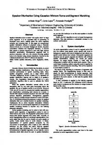
Figure 1. A comparison of the methods using the three primary techniques discussed for reducing a 10 component Gaussian mixture to 5 components. Note that the line for the brute force approach overlaps that of the optimal solution most of the time.
4) Once the final bin containing lb items has been filled and S updated, if the current bin is not the final bin, continue assigning things to the subsequent bins (which will each hold fewer than Ib items) either using the method for when there are no repeats or the method for repeats, as appropriate. In order to ensure that we get the best possible estimate for comparison, we will use the iterative optimization of Section III-C to refine this brute-force estimate when simulating. V. S IMULATIONS
COWA Runnalls GMRC Brute Force
ISE
NISE
0.1165 0.0834 0.0482 0.0359
0.1080 0.0814 0.0432 0.0309
Execution Time (sec) 0.0390 0.0048 53.4499 622.0235
Table I T HE PERFORMANCE AND EXECUTION TIMES OF THE FOUR METHODS IN THE 4- DIMENSIONAL RANDOMIZED REDUCTION SCENARIO REDUCING A 10 COMPONENT MIXTURE TO 5 COMPONENTS . T HE RESULTS ARE AVERAGED OVER 500 M ONTE C ARLO RUNS .
We compared the performance of the modified GMRC and COWA algorithms described in Section III against the brute force approach of Section IV and against simply using Runnalls’ algorithm (the first step of the GMRC). The simulation was run reducing randomly generated D = 4 dimensional N = 10 component Gaussian mixtures to L = 5 component mixtures, meaning that the brute-force approach had to calculate the cost of 42, 525 possible reductions each time. The COWA algorithm was run with γ = ∞ and � = 0, forcing the algorithm to reduce the mixture to the minimum number of components each time. The components of the means were chosen uniformly between 0 and 3. The covariances of the mixture components were chosen from a 1 I and 5 degrees Wishart distribution [31] with scale matrix 50 of freedom. The mean covariance for each component was
1 I. The weights for the components were chosen from thus 10 a symmetric Dirichlet distribution [32] with parameter α = 1. The execution times of the algorithms and their performance in terms of the normalized integral squared difference, as defined in Equation (17), which ranges from zero to one (smaller numbers are better) is given in Table I. The simulation was run on a 2.4GHz computer running the Mac OS X version of MATLAB. From Table I, we can see that the COWA lags behind the faster, lower-complexity algorithm by Runnalls. The improvement over Runnalls’ algorithm by the GMRC comes at a steep computational cost. All algorithms have room for improvement in terms of ISE and ISE compared to the slow, brute-force algorithm. To better visualize the performance of the reduction algorithms, we considered a scalar scenario using the following parameters:
w ={0.03, 0.18, 0.12, 0.19, 0.02, 0.16, 0.06, 0.1, 0.08, 0.06} µ ={1.45, 2.20, 0.67, 0.48, 1.49, 0.91, 1.01, 1.42, 2.77, 0.89} P ={0.0487, 0.0305, 0.1171, 0.0174, 0.0295, 0.0102, 0.0323, 0.0380, 0.0115, 0.0679} The 10-component mixture was reduced to five components using the COWA, the GMRC and the brute-force algorithm. The result is shown in Figure 1. We can see that the reduced mixture using the brute-force reduction approach is the only method that avoids large deviations from the original mixture. However, to what extent does this matter in a practical algorithm? To address this question, we implemented Salmond’s [6] Gaussian mixture reduction-based tracking algorithm using the COWA and the GMRC. We considered tracking a single target in 2D using the standard motion model used with the Kalman filter, namely xt (k + 1) =F (k)xt (k) + vt (k) zt (k) =Ht (k)xt (k) + wt (k)
(43) (44)
where x is the state, z is a Cartesian position measurement and vt and wt are independent Gaussian white noise. We used a sampling interval of τ = 1s. We maintained L = 3 hypotheses across time-steps. We used the discretized continuous time white noise acceleration model from [9] with process noise parameter q = 2. The target started at the origin having an initial velocity of 10 m/s in both Cartesian components. The measurement covariance was a diagonal matrix with 60 on both of the diagonal elements. The probability of detecting the target was 70%. Rectangular gates enclosing the 99.9% confidence region (which is elliptical) were used about each hypothesized target state. Clutter was generated in the gate according to a Poisson distribution having density λ = 5.6 × 10⁻⁵ . The number of clutter points in each gate varied, but were often around 1−5. The initial state was determined using two measurements from the true target. The trackers were run for 1000 Monte Carlo runs for a maximum of 50-time steps. Table II shows the percentage of lost tracks as a function of the tracker used as well as the RMSE of the tracks that were not lost. Tracks were declared lost if the true target location
RMSE COWA Runnalls GMRC
9.11 7.98 8.26
% Lost Tracks 25.35 3.15 3.25
Table II T HE PERCENTAGE OF LOST TRACKS OVER A 50- STEP PERIOD , AS WELL AS THE RMSE OF THE TRACKS THAT WEREN ’ T LOST, AS A FUNCTION OF THE MIXTURE REDUCTION ALGORITHM USED IN IMPLEMENTATIONS OF S ALMOND ’ S TRACKER WITH L = 3 HYPOTHESES KEPT.
was not in any of the gates at a particular time-step or if no hypotheses were left. Hypotheses were declared lost and were subsequently pruned if the gate for any of them exceeded 500 meters in either dimension. We can see that the quality of the reduction algorithm is important, with Runnalls’ algorithm and the GMRC having significantly fewer lost tracks than the COWA. However, there is no noticeable improvement between the Runnalls’ algorithm and the GMRC. VI. C ONCLUSIONS In Section III-C, it was noted that the accepted optimization of the weight terms in the GMRC and COWA algorithms could result in the reduced Gaussian mixture being invalid. We have made an appropriate modification to address this. We also combined concepts from other papers, generalizing the GMRC to vector distributions. To form a basis for comparison with other algorithms, we derived a brute-force approach. From the simulations using random Gaussian mixtures, we can see that the GMRC is the best algorithm (in terms of ISE) in comparison to the brute force algorithm. Indeed, the COWA was inferior to Runnalls algorithm both in performance as well as execution time. However, the improvement in running the full GMRC versus simply running the first step (Runnalls’ algorithm) is nonexistent when looking at a tracking scenario, suggesting that a naked Runnalls’ algorithm would be the most practical Gaussian mixture reduction algorithm to use in a tracker thus far. R EFERENCES [1] B. Krukowski and J. Dauwels, “Message passing decoding of lattices using Gaussian mixtures,” in Proceedings of the IEEE International Symposium on Information Theory, Toronto, ON, Canada, Jul. 2008, pp. 2489–2493. [2] A. Nikseresht and M. Gelgon, “Gossip-based computation of a Gaussian mixture model for distributed multimedia indexing,” IEEE Trans. Multimedia, vol. 10, no. 3, pp. 385–392, Apr. 2008. [3] H. Chen, K. C. Chang, and C. Smith, “Constraint optimized weight adaptation for Gaussian mixture reduction,” in Proceedings of SPIE: Signal Processing, Sensor Fusion, and Target Recognition XIX, vol. 7697, Orlando, FL, Apr. 2010, pp. 76 970N–1–76 970N–10. [4] P. Bruneau, M. Gelgon, and F. Picarougne, “Parsimonious reduction of Gaussian mixture models with a variational-Bayes approach,” Pattern Recognition, vol. 43, no. 3, pp. 850–858, Mar. 2010. [5] S. S. Blackman, “Multiple hypothesis tracking for multiple target tracking,” IEEE Aerosp. Electron. Syst. Mag., vol. 19, no. 1, pp. 5–18, Jan. 2004. [6] D. J. Salmond, “Mixture reduction algorithms for point and extended object tracking in clutter,” IEEE Trans. Aerosp. Electron. Syst., vol. 45, no. 2, pp. 667–686, Apr. 2009. [7] ——, “Mixture reduction algorithms for target tracking in clutter,” in Proceedings of SPIE: Signal and Data Processing of Small Targets Conference, vol. 1305, Oct. 1990, pp. 434–445.
[8] L. Y. Pao, “Multisensor mixture reduction algorithms for tracking,” Journal of Guidance, Control and Dynamics, vol. 17, no. 6, pp. 1205– 1211, Nov.–Dec. 1994. [9] Y. Bar-Shalom, P. K. Willett, and X. Tian, Tracking and Data Fusion. YBS Publishing, 2011. [10] D. J. Petrucci, “Gaussian mixture reduction for Bayesian target tracking in clutter,” Master’s thesis, Air Force Institute of Technology, Dec. 2005. [Online]. Available: http://www.dtic.mil/srch/doc?collection= t3&id=ADA443588 [11] D. W. Scott, “Parameter modeling by minimum L2 error,” Department of Statistics, Rice University, Tech. Rep. 98-3, Feb. 1999. [Online]. Available: http://www.stat.rice.edu/∼scottdw/ftp/l2e.r1.ps [12] D. W. Scott and W. F. Szewczyk, “From kernels to mixtures,” Technometrics, vol. 43, no. 3, pp. 323–335, Aug. 2001. [13] J. E. Harmse, “Reduction of Gaussian mixture models by maximum similarity,” Journal of Nonparametric Statistics, vol. 22, no. 6, pp. 703– 709, Dec. 2009. [14] J. L. Williams and P. S. Maybeck, “Cost-function-based hypothesis control techniques for multiple hypothesis tracking,” Mathematical and Computer Modelling, vol. 43, no. 9–10, pp. 976–989, May 2006. [15] J. L. Williams, “Gaussian mixture reduction for tracking multiple maneuvering targets in clutter,” Master’s thesis, Air Force Institute of Technology, Mar. 2003. [Online]. Available: http://www.dtic.mil/srch/ doc?collection=t3&id=ADA415317 [16] M. Rosenblatt, “Remarks on some nonparametric estimates of a density function,” The Annals of Mathematical Statistics, vol. 27, no. 3, pp. 832–837, Sep. 1956. [17] M. West, “Approximate posterior distributions by mixture,” Journal of the Royal Statistical Society. Series B (Methodological), vol. 55, no. 2, pp. 409–422, 1993. [18] M. F. Huber and U. D. Hanebeck, “Progressive Gaussian mixture reduction,” in Proceedings of the 11th International Conference on information Fusion, Cologne, Germany, Jan. 2008, pp. 1–8. [19] O. C. Schrempf, O. Feiermann, and U. D. Hanebeck, “Optimal mixture approximation of the product of mixtures,” in Proceedings of the Eighth International Conference on information Fusion, Philadelphia, PA, Jul. 2005, pp. 85–92. [20] D. Schieferdecker and M. F. Huber, “Gaussian mixture reduction via clustering,” in Proceedings of the 11th International Conference on information Fusion, Seattle, WA, Jul. 2009, pp. 1536–1543. [21] A. R. Runnalls, “Kullback-Leibler approach to Gaussian mixture reduction,” IEEE Trans. Aerosp. Electron. Syst., vol. 43, no. 3, pp. 989–999, Jul. 2007. [22] K. C. Chang and W. Sun, “Scalable fusion with mixture distributions in sensor networks,” in Proceedings of the 11th International Conference on Control, Automation, Robotics, and Vision, Singapore, Dec. 2010, pp. 1251–1256. [23] C. Bishop, Pattern Recognition and Machine Learning. Cambridge, U.K.: Springer, 2006. [24] T. Kanungo, D. M. Mount, D. S. Netanyahu, C. D. Piatko, R. Silverman, and A. Y. Wu, “An efficient k-means clustering algorithm: Analysis and implementation,” IEEE Trans. Pattern Anal. Mach. Intell., vol. 24, no. 7, pp. 881–892, Jul. 2002. [25] D. Bertsekas, Nonlinear Programming, 2nd ed. Belmont, Massachusetts: Athena Science, 2003. [26] G. H. Golub and C. F. Van Loan, Matrix Computations, 3rd ed. Baltimore: Johns Hopkins University Press, Oct. 1996. [27] D. Bertsimas and J. N. Tsitsiklis, Introduction to Linear Optimization, 1st ed. Belmont, Massachusetts: Athena Science, Feb. 1997. [28] D. Aloise, “Exact algorithms for minimum sum-of-squares clustering,” ´ Ph.D. dissertation, Ecole Polytechnique de Montr´eal, Jun. 2009. [Online]. Available: http://www.gerad.ca/∼aloise/These.pdf [29] R. E. Jensen, “A dynamic programming algorithm for cluster analysis,” Operations Research, vol. 17, no. 6, pp. 1034–1057, Nov.–Dec. 1969. [30] E. W. Weisstein, CRC Concise Encyclopedia of Mathematics. Boca Raton: CRC Press, 1999, p. 1741. [31] M. L. Eaton, Multivariate Statistics: A Vector Space Approach, ser. Institute of Mathematical Statistics Lecture Notes-Monograph Series. Beachwood, Ohio: Institute of Mathematical Statistics, 2007, vol. 53, ch. 5 & 8. [32] B. A. Frigyik, A. Kapila, and M. R. Gupta, “Introduction to the Dirichlet distribution and related processes,” University of Washington, Tech. Rep. UWEETR-2010-0006, Dec. 2010. [Online]. Available: https://www.ee. washington.edu/techsite/papers/refer/UWEETR-2010-0006.html