Gaussian Mixture Approximation by Another ... - Semantic Scholar

AIAA 2010-7747

AIAA Guidance, Navigation, and Control Conference 2 - 5 August 2010, Toronto, Ontario Canada

Gaussian Mixture Approximation by Another Gaussian Mixture for "Blob" Filter Re-Sampling Mark L. Psiaki∗, Jonathan R. Schoenberg# Cornell University, Ithaca, N.Y. 14853-7501 and Isaac T. Miller Coherent Navigation, Inc., San Mateo, CA 94404

A new method has been developed to approximate one Gaussian mixture by another in a process that generalizes the idea of importance re-sampling in a particle filter. This algorithm is being developed as part of an effort to generalize the concept of a particle filter. In a traditional particle filter, the underlying probability density function is described by particles: Dirac delta functions with infinitesimal covariances. This paper develops an important component of a “blob” filter, which uses a Gaussian mixture of “fattened,” finitecovariance blobs instead of infinitesimal particles. The goal of a blob filter is to save computational effort for a given level of probability density precision by using many fewer blobs than particles. Most of the techniques necessary for this type of filter have already been developed. The one missing component is developed in this paper: a re-sampling algorithm that bounds the covariance of each element while accurately re-producing the original probability distribution. The covariance bounds are needed in order to keep the blobs from becoming too “fat”; otherwise, Extended Kalman Filter (EKF) or Unscented Kalman Filter dynamic propagation and measurement update calculations would cause excessive truncation error for each blob. The re-sampling algorithm is described in detail, and its performance is studied using several simulated test cases. Also discussed is the usefulness of a Gaussian mixture and EKF-like techniques for nonlinear dynamic propagation and nonlinear measurement update of probability distributions.

I. Introduction

D

ifficulties can arise when solving certain nonlinear dynamic estimation problems. The default solution algorithm for such problems is the EKF, but the EKF has a known potential to diverge or to yield sub-optimal accuracy 1,2,3. Various algorithms have been developed with the goal of improved convergence robustness or accuracy in the presence of strong nonlinearities, among them the Unscented or Sigma-Points Kalman Filter (UKF) 1,4 , the Particle Filter (PF) 2, and the Backward-Smoothing Extended Kalman Filter 3. The PF is attractive for its simplicity and its theoretical guarantee of convergence to the optimal result in the limit of very many particles. The required number of particles to achieve a reasonable result, however, can become overwhelming for state space dimensions as small as 3 or 4, as in Ref. 5. A sensible generalization of the PF is to use Gaussian mixtures to represent probability density functions. In effect, a PF works with representations of probability density functions that are sums of Dirac delta functions. A Gaussian mixture generalizes this concept by using elements that have finite widths instead of infinitesimal widths. A sum of finite-width elements has the potential to approximate a probability density function with many fewer elements than would be needed by a PF for the same degree of accuracy, as measured based on differences of multiple moments or based on the functional norm "distance" from the true probability density. Thus, a Gaussian mixture filter has the potential to solve the curse of dimensionality that causes a PF to become impractical for state space dimensions above 2 or 3. ∗ #

Professor, Sibley School of Mechanical and Aerospace Engineering. Associate Fellow, AIAA. Graduate student, Sibley School of Mechanical and Aerospace Engineering. 1 American Institute of Aeronautics and Astronautics

Copyright © 2010 by Mark L. Psiaki, Jonathan R. Schoenberg, & Isaac T. Miller. Published by the American Institute of Aeronautics and Astronautics, Inc., with permission.

Gaussian mixture filters have been studied extensively in the past, and Ref. 6 is one of the earliest known papers on this subject. The proposed "blob" filter is a modified version of the Gaussian mixture filter of Ref. 7. That filter implements a separate standard UKF dynamic propagation and measurement update for each element of its Gaussian mixture. Its approximate implementation of the full non-linear Bayesian measurement update dictates that it recalculate the weights of its mixture elements. This re-calculation increases the weights of elements whose predicted measurements best match the actual measurement at the given sample, as in the static multiple-model filter described in Ref. 8. The final filter action for a given sample is to re-approximate the mixture by drawing samples from it and then fitting a new Gaussian mixture to the samples. This action can avert degeneracy of the mixture into one element or a very few elements that have appreciable weight, and it can reduce the number of elements in cases where the multiplication of Gaussian mixtures would cause exponential growth of this number. The Gaussian mixture filter of Ref. 7 has strengths and weaknesses. Its main strength lies in the potential accuracy of the UKF dynamic propagation and measurement update of the mixture. If each element of the Gaussian mixture has a covariance that is sufficiently small, as measured in terms of the maximum eigenvalue or some other sensible metric, then the UKF calculations will be very accurate. With sufficiently small covariances, EKF calculations also would be sufficiently accurate to yield a good estimate of the posterior probability density function. This is true because a narrow distribution implies good accuracy of the Taylor series approximations inherent in the UKF or EKF calculations. That is, the Taylor series approximations are accurate over the likely ranges of state variations of each mixture element. The weakness of the filter of Ref. 7 lies in its re-approximation of the Gaussian mixture distribution after the measurement update. This re-approximation samples the original mixture and fits a new Gaussian mixture to the samples via Expectation Maximization (EM). This procedure achieves the worthy goal of eliminating mixture elements with low weights. Unfortunately, it does not limit the maximum covariance of any element of the reapproximation. This limitation is needed so that the next recursion of the filtering algorithm will yield good accuracy when using the approximations that are inherent in its element-by-element EKF or UKF calculations. It is not obvious how to add such a limitation to the EM-based re-sampling procedure without making it unduly complicated. The other weakness of the mixture re-approximation is its failure to fit the old mixture as closely as possible in some functional norm sense, as in the Integral Square Difference (ISD) metric of Ref. 9. Instead, the filter of Ref. 7 uses an ad hoc transition first to particle samples of the old mixture and finally back to Gaussian mixture elements that fit these particles. Section IV of Ref. 10 constitutes a prototype application of similar concepts to those of Ref. 7, albeit with EKFs used in place of UKFs for propagating and updating the Gaussian mixture elements and without any need for re-sampling. The goal of this application was to achieve filter convergence from large initial uncertainty in a difficult spacecraft attitude determination problem. The algorithm converged reliably from large initial errors that would have caused an EKF to fail. This reliable convergence implies that the algorithm of Ref. 7 could provide a powerful solution to difficult problems in nonlinear filtering if it were modified to use this paper's re-sampling procedure. The present paper's contribution is an improved Gaussian mixture re-approximation algorithm that could be applied to a filter like that of Ref. 7. It has four important properties: First, it chooses elements of the new mixture so that their covariances lie below a linear matrix inequality (LMI) upper bound. This constraint is included to ensure that element-by-element EKF or UKF dynamic propagation and measurement update calculations will yield a sufficiently accurate approximation of the a posteriori probability density function on the next Bayesian filter step. Second, it directly chooses new mixture elements and their weights in a way that seeks to minimize the ISD between the new Gaussian mixture distribution and the original distribution. Third, it tends not to waste new elements in attempts to approximate the contributions of original elements that have low weights. Last, it tends to hold down the number of needed new elements through a combination of strategies. These strategies include a) maximization of new element covariances subject to the LMI constraint, b) selection of new element means and weights in a way that tends to limit the number of new elements needed for a given improvement to the ISD, c) termination of the generation of new elements when a conservative upper bound has been met for the ISD between the new and old mixtures, and d) combination of elements if their Gaussian sum can be approximated well by a single new element. There exist other Gaussian mixture re-sampling schemes 9,11,12. This paper's new algorithm differs from the existing algorithms in several important respects. The existing algorithms' primary goal is to approximate an original mixture by a new one that has fewer elements. The present algorithm retains this as a secondary goal, but its main goal is to develop a new approximate mixture whose elements all have covariances that satisfy an LMI

2 American Institute of Aeronautics and Astronautics

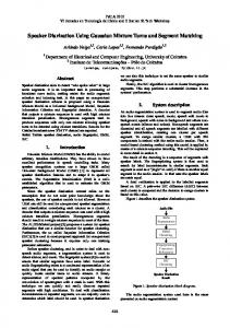
upper bound, which is an important property when using Gaussian mixtures to generalize nonlinear particle filtering. The new algorithm uses the ISD fit metric of Ref. 9, but in a new way: It formulates and solves quadratic programs based on the ISD metric in order to choose optimal relative weights for subsets of the new mixture's elements. This paper's new Gaussian mixture re-approximation method will be useful for generalizing the nonlinear particle filter to create a blob filter along the lines of Ref. 7, as stated above. The key generalization is to replace particles of infinitesimal width by blobs of finite width. Therefore, another important aspect of the new reapproximation scheme is that it approaches the re-sampling scheme of a standard particle filter 2 in the limit of a very small upper bound on the covariances of the new elements. This asymptotic similarity makes the blob filter a natural generalization of the particle filter. Asymptotic similarity to PF re-sampling is achieved by choosing the mean values of the new mixture elements through the use of a modified sampling method. This modified procedure employs a perturbation of the original distribution, and it samples the perturbed distribution using Metropolis-Hastings techniques 13. The perturbed distribution reduces the original distribution near existing new elements, thereby reducing the probability that additional new elements will be located near existing elements. A particle filter, on the other hand, tends to sample many particles very near each other in regions of the filter's state space that have high probability densities, as characterized by the high numbers of existing particles in those regions. The new re-sampling method achieves equivalent results through an explicit increase of the weights that it assigns to new mixture elements that lie in regions of high original probability density. Figure 1 depicts the new re-sampling algorithm in block-diagram form. It starts in the upper left-hand corner of the diagram with original Gaussian mixture distribution pa(x). Its 1st block decomposes pa(x) into sub-mixtures, and its remaining blocks fit corresponding sub-mixtures of the new re-sampled distribution to these original submixtures. Initially, each sub-mixture of the new distribution is a poor fit to the corresponding sub-mixture of the original distribution because it lacks elements, and the algorithm initializes fit parameters accordingly in its 2nd block. Each new sub-mixture uses a common covariance matrix for each of its elements, and the set of sub-mixture covariance matrices is computed in the 3rd algorithm block. The 3rd block also pre-computes parameters that are used in the 7th block in order to set up an optimization problem for the relative weights within each new submixture. The algorithm's main loop is depicted by the 4th-10th blocks of Fig. 1. It adds one new element to the new Gaussian mixture per pass through these blocks. The 4th block computes modified sub-mixture weights that assign higher values to those original sub-mixtures that have a) high original weights, b) poor fits to their corresponding new sub-mixtures, or c) both. The 5th block picks which new sub-mixture to augment with a new element. The selection procedure uses importance sampling and the modified weights from the 4th block. A new sub-mixture is likely to gain a new element if its corresponding original sub-mixture has a sufficiently high original weight and if its fit to that original sub-mixture is sufficiently poor. The 6th block draws the mean value of the new mixand from a modified form of the probability density function of the corresponding original sub-mixture. This modified submixture has reduced probability density near pre-existing new sub-mixture elements, thereby reducing the likelihood of close spacing between new elements. The 7th block optimizes the relative weights of the new submixture to account for its new mixand. Decision block 8 rejects the new mixand if the resulting ISD fit error of the augmented sub-mixture does not decrease, in which case another new-element mean value is sampled in a return to the 6th block. Otherwise, two termination criteria are tested in the 9th and 10th blocks. Termination occurs if the overall fit error is sufficiently small or if a given upper limit on the number of new mixands has been reached. The 11th block finishes by computing the new mixands' final weights. This paper develops and analyzes its new Gaussian mixture re-approximation algorithm in 8 main sections. Section II defines Gaussian mixtures using square-root information matrix notation, and it defines sub-mixtures as being subsets of the elements of a given mixture. Section III develops the ISD error metric between two Gaussian mixtures, derives an analytic formula for the ISD, and determines an upper bound for the relative norm error between two Gaussian mixtures. This relative upper bound is used to implement the algorithm termination test in the 9th block of Fig. 1. Section IV presents a quadratic program (QP) that chooses the weights of a new Gaussian mixture in order to minimize the ISD between it and an original Gaussian mixture. This QP algorithm is used in the 7th block of Fig. 1. Section V defines an LMI that bounds the covariances of the elements of the new Gaussian mixture. It develops an algorithm for choosing the covariance of a new element in a way that respects this limit while deviating as little as possible from the covariance of a corresponding element of the original mixture. This LMI solution algorithm is used by the 3rd block of Fig. 1. Section VI introduces a technique for decomposing the original mixture into sub-mixtures, as per Block 1 of Fig. 1. These sub-mixture groupings can help to reduce the


number of elements of the new mixture. Section VII presents the algorithm for selecting means and covariances of new mixture elements, as needed to implement the 6th block in Fig. 1. Section VIII combines the developments of Sections II-VII in order to define the new Gaussian mixture re-sampling algorithm. Section IX presents example test results that illustrate the performance and usefulness of the new algorithm. Section X summarizes this paper's developments and presents its conclusions. Start

3

2

1 Decompose pa(x) into original submixtures & initialize corresponding new sub-mixtures as empty sets

4

Pre-compute new sub-mixture covariances that satisfy LMIs along with quantities used to set up weight optimizations

Initialize sub-mixture fit parameters to indicate poor fits

Compute modified submixture weights based on weights of original sub-mixtures & on current sub-mixture fit parameters 7

5 Draw mean of new element of corresponding new sub-mixture from modified original submixture distribution & use precomputed new covariance to define new sub-mixture element

Do importance sampling based on modified weights to pick an original submixture with relatively poor current fit/relatively high original weight

Re-optimize relative weights within corresponding new sub-mixture to minimize ISD from original sub-mixture & update new sub-mixture's fit parameter 6

8

9

Sub-mixture ISD decrease?

Sufficiently good fit to all of pa(x)?

No

Yes

10

Yes

11

No

Reached limit on No. of new mixands?

No

Yes

Compute new mixand weights based on new sub-mixture weights & on optimized relative weights within new sub-mixtures

Stop

Fig. 1. Flow chart of Gaussian mixture re-sampling algorithm.

II. Gaussian Mixture Probability Density Functions A. Original and New Gaussian Mixture Probability Density Functions A Gaussian mixture is a weighted sum of Gaussian distributions. The ith element of the mixture, also called the ith mixand or the ith component, can by characterized by its square-root information matrix Ri and its mean μi. The element probability distribution is: N sr ( x; μ i , Ri ) =

| det( Ri ) |

T

e −0.5[ Ri ( x − μi )]

[ Ri ( x − μi )]

= N ( x; μ i , Ri−1 Ri−T )

(1) (2π ) where x and μi are n-dimensional vectors and Ri is an n-by-n matrix. The covariance matrix of this distribution is Pi = Ri−1 Ri−T , where the notation ()-T indicates the inverse of the transpose of the matrix in question. The notation N(x;μ,P) indicates the usual normal distribution in the vector x that has mean μ and covariance matrix P. The new notation Nsr(x;μ,R) indicates the same distribution in x, except that its covariance is characterized by the square-root information matrix R in place of the covariance matrix P. This non-standard parameterization of the normal n/2


distribution will be used throughout the remainder of this paper. It has been chosen because it allows a simple LMI solution in Section V and because it is consistent with the planned square-root information filter (SRIF) implementation of the proposed “blob” filter. An SRIF implementation is desirable because it has good numerical stability. Each element of a Gaussian mixture also has a weight, wi. Each weight must be non-negative. The sum of all of the weights equals 1. If there are N elements in the mixture, then N

1 = ∑ wi and wi ≥ 0 for i = 1, ..., N

(2)

i =1

Given the Gaussian component definition in Eq. (1) and weights that obey the constraints in Eq. (2), the corresponding Gaussian mixture is N

p gm ( x; w1 , μ1 , R1 ,..., w N , μ N , R N ) = ∑ wi N sr ( x; μ i , Ri )

(3)

i =1

It is straightforward to show that this probability density function preserves the unit normalization constraint and that its mean and covariance are, respectively, N

μ gm = ∑ wi μ i i =1

N

and Pgm = ∑ wi [ Ri−1 Ri−T + ( μ i - μ gm )( μ i - μ gm ) T ] i =1

(4)

It is necessary to distinguish between two Gaussian mixture distributions in this paper. Suppose that one distribution, distribution "a", is characterized by the weights, mean values, and square root-information matrices wai, μai, Rai for i = 1, ..., Na. Similarly, suppose that another related distribution, distribution "b", is characterized by wbj, μbj, Rbj for j = 1, ..., Nb. The following short-hand notation is used to indicate these two distributions Na

p a ( x ) = p gm ( x; wa1 , μ a1 , R a1 ,..., waN a , μ aN a , R aN a ) = ∑ wai N sr ( x; μ ai , R ai )

(5a)

p b ( x ) = p gm ( x; wb1 , μ b1 , Rb1 ,..., wbNb , μ bNb , R aNb ) = ∑ wbj N sr ( x; μ bj , Rbj )

(5b)

i =1 Nb j =1

The goal of this paper is to develop a method that picks the parameters of distribution "b", Nb and wbj, μbj, and Rbj for j = 1, ..., Nb. It seeks to pick these parameters in a way that will cause pb(x) to be a good approximation of pa(x) while respecting an LMI lower bound on every RbjTRbj for j = 1, ..., Nb. The algorithm's LMI lower bound on −1 −T RbjTRbj is an alternate means of enforcing an LMI upper bound on the covariance Pbj = Rbj Rbj . The algorithm also seeks to keep the number of new elements Nb from being too large. Of course, there normally is a trade-off between the size of Nb and the accuracy with which pb(x) approximates pa(x).

B. Decomposition into Sub-Mixtures It can be useful to break Gaussian mixtures pa(x) and pb(x) into weighted sums of sub-mixtures. This decomposition allows the original function approximation problem to be broken into a set of smaller approximation problems. It can be used to reduce the computational burden of this paper's algorithms. Note that the term “submixture” is non-standard. It denotes a Gaussian mixture distribution that is formed using a re-weighted subset of the elements of an original Gaussian mixture. Let distribution pa(x) and distribution pb(x) be broken into the following disjoint sets of sub-mixtures ihim

∑ wai N sr ( x; μ ai , R ai )

p sam ( x ) =

i =ilom

for m = 1, ..., M

(6a)

for m = 1, ..., M w sbm where the sub-mixture cumulative weights are defined to be

(6b)

w sam jhim

∑

p sbm ( x ) =

j = jlom

ihim

wsam = ∑ wai i =ilom

wbj N sr ( x; μ bj , Rbj )

for m = 1, ..., M


(7a)

wsbm =

j him

∑

j = j lom

wbj

for m = 1, ..., M

(7b)

The start and stop indices ilom and ihim define the index range of components of the original Gaussian mixture pa(x) that form its mth sub-mixture psam(x). The indices jlom and jhim work similarly to define the mth sub-mixture psbm(x) of pb(x). These indices obey the constraints: ilo1 = 1, jlo1 = 1,

ilo(m+1) = ihim+1 for m = 1,...,(M-1), jlo(m+1) = jhim+1 for m = 1,...,(M-1),

ihiM = Na, jhiM = Nb,

and ilom ≤ ihim for m = 1,...,M and jlom-1 ≤ jhim for m = 1,...,M

(8a) (8b)

These index constraints ensure that each original mixand appears in one and only one sub-mixture for probability density functions pa(x) and pb(x). The mth sub-mixture of pa(x) has Nam = ihim - ilom+1 Gaussian components, and the mth sub-mixture of pb(x) has Nbm = jhim - jlom+1 components. The constraint jlom-1 ≤ jhim allows for the possibility that Nbm = 0 if jlom-1 = jhim. In this situation, psbm(x) and wsbm are undefined. This situation may arise if the corresponding original sub-mixture weight wsam is very low, in which case the new Gaussian mixture pb(x) may not devote any elements to fitting the effects of psam(x). It is helpful to define relative weights within a given sub-mixture. They are: ( wai = wai / w sam for i = ilom, ..., ihim and for m = 1, ..., M (9a) ( for j = jlom, ..., jhim and for m = 1, ..., M (9b) wbj = wbj / w sbm Equations (9a) and (9b) guarantee normalization of the weights within each sub-mixture, and they allow the submixtures in Eqs. (6a) and (6b) to be expressed as true Gaussian mixtures in their own right: ihim ( p sam ( x ) = ∑ wai N sr ( x; μ ai , Rai ) for m = 1, ..., M (10a) i =ilom

p sbm ( x ) =

jhim

∑

j = jlom

( wbj N sr ( x; μ bj , Rbj ) for m = 1, ..., M

(10b)

It is possible to express the two original Gaussian mixtures as weighted sums of these sub-mixtures: M

pa ( x ) = ∑ wsam psam ( x )

(11a)

pb ( x ) = ∑ wsbm psbm ( x )

(11b)

m =1 M

m =1

Equations (7a) and (7b) and the normalization and non-negativeness of the original mixture weights imply that the sub-mixture weights are also normalized and non-negative: M

1 = ∑ wsam

and wsam ≥ 0 for m = 1, ..., M

(12a)

1 = ∑ wsbm

and wsbm ≥ 0 for m = 1, ..., M

(12b)

m =1 M

m =1

III. The Integral Square Difference between Two Gaussian Mixtures as a Measure of Approximation Accuracy A. ISD Definition The Integral Square Difference is a good measure of the accuracy with which pb(x) approximates pa(x). The ISD is defined to be the integral of the square of the difference between these two probability density functions 9: ∞

J ISD = ∫ [ pa ( x ) − pb ( x )]2 dx

(13)

−∞

This quantity is non-negative, and its square root is the functional 2-norm of the difference between the probability distributions || pa ( x ) − pb ( x ) ||2 = J ISD

⎧∞ ⎫ = ⎨ ∫ [ pa ( x ) − pb ( x )]2 dx ⎬ ⎩− ∞ ⎭

0.5


(14)

Therefore, the ISD is a good measure of the similarity between these two functions. A very small value of the ISD cost JISD indicates that pb(x) is a very good approximation of pa(x). Distribution pb(x) perfectly matches pa(x) if and only if JISD = 0. Some re-approximation algorithms seek to choose pb(x) in a way that explicitly constrains the mean and covariance of the new distribution to equal that of pa(x), e.g., see Ref. 11. In order to avoid an additional source of algorithmic complexity, the current approach enforces no such constraint. If JISD in Eq. (13) is sufficiently small, however, then the mean and covariance of pb(x) will be very close to the corresponding pa(x) quantities, as demonstrated by example in Section IX. In addition, a small JISD could cause a number of higher moments of pb(x) to be closer to the corresponding moments of pa(x) than they would be if a different re-approximation technique were used to construct pb(x) without consideration of its JISD.

B. Analytic Formulas for the ISD Reference 9 presents analytic formulas for evaluating the integral in Eq. (13). The formulas used here are modified versions of those found in Ref. 9. The modifications account for the use of square-root information matrices in place of mixand covariance matrices. Suppose that one defines weight vectors for the two probability density functions: wa = [wa1;wa2;wa3;...;waNa] and wb = [wb1;wb2;wb3;...;wbNb]. Then the integral in Eq. (13) can be written as a quadratic form in these two vectors: J ISD = w aT H aa w a − 2 w aT H ab wb + wbT H bb wb

(15)

where Haa, Hab, and Hbb are matrices with the respective dimensions Na-by-Na, Na-by-Nb, and Nb-by-Nb. The matrices Haa and Hbb are symmetric and at least positive semi-definite. The elements of these matrices can be evaluated using the formulas: ∞

[ H aa ]ik = ∫ N sr ( x; μ ai , Rai )N sr ( x; μ ak , Rak )dx

for i = 1,...,Na and k = 1,...,Na

(16a)

[ H ab ]ij = ∫ N sr ( x; μ ai , Rai )N sr ( x; μbj , Rbj )dx

for i = 1,...,Na and j = 1,...,Nb

(16b)

[ H bb ] jl = ∫ N sr ( x; μbj , Rbj )N sr ( x; μbl , Rbl )dx

for j = 1,...,Nb and l = 1,...,Nb

(16c)

−∞ ∞

−∞ ∞

−∞

where the notation []ik indicates the row-i/column-k element of the matrix in question. The integrals in Eqs. (16a)-(16c) can be evaluated analytically by using the normalization property of a Gaussian distribution and the fact that the product of two Gaussian distributions is itself a Gaussian distribution, although not properly normalized 9. These integrals take the general form: ∞ | det( Rc ) || det( Rd ) | − 0.5[ R~cd ( μ c − μ d )]T [ R~cd ( μ c − μ d )] e (17) ∫ N sr ( x; μc , Rc )N sr ( x; μ d , Rd )dx = (2π ) n / 2 | det( Rcd ) | −∞ ~ where the n-by-n matrices Rcd and Rcd are computed based upon the following orthonormal/upper-triangular (QR) factorization 14: ⎡R ⎤ ⎡ R ⎤ ⎡R ⎤ Q ⎢ cd ⎥ = [Q1 , Q2 ]⎢ cd ⎥ = ⎢ c ⎥ (18) 0 ⎣ 0 ⎦ ⎣ Rd ⎦ ⎦ ⎣ with Q being a 2n-by-2n orthonormal matrix and Rcd an n-by-n upper-triangular matrix. Q1 equals the first n columns of Q, and Q2 equals the last n columns. These matrices are used to compute

⎡0⎤ ⎡R ⎤ ~ Rcd = Q2T ⎢ c ⎥ = −Q2T ⎢ ⎥ 0 ⎣ ⎦ ⎣ Rd ⎦

(19)

Equations (17)-(19) have been derived using a lengthy, non-intuitive sequence of matrix/vector manipulations that have been omitted for the sake of brevity. In the special case where Rc = Rd, it suffices to use Rcd = 2 Rc and ~ Rcd = (1 / 2 ) Rc , and in this case the Eq. (17) integral becomes ∞ | det( Rc ) | − 0.25[ Rc ( μ c − μ d )]T [ Rc ( μ c − μ d )] e (20) ∫ N sr ( x; μ c , Rc )N sr ( x; μ d , Rc )dx = 2n π n / 2 −∞


C. An ISD-Based Metric for Relative Fit Error The ISD formula in Eq. (15) can be used to develop a relative measure of the accuracy with which new Gaussian mixture pb(x) approximates original Gaussian mixture pa(x). A sensible metric is the norm of the difference between pb(x) and pa(x) divided by the norm of pa(x): erelba =

|| pa ( x ) − pb ( x ) ||2 = || pa ( x ) ||2

w aT H aa w a − 2w aT H ab wb + wbT H bb wb

(21)

w aT H aa w a

If this quantity is small relative to 1, then the difference between pb(x) and pa(x) is small relative to the magnitude of pa(x). The metric erelba provides a sensible termination criterion for the procedure that generates new mixand elements of pb(x). If erelba is sufficiently small compared to 1, then the algorithm should terminate with the given pb(x); otherwise, it should continue generating new elements. If erelba is very small compared to 1, then the mean and covariance of pb(x) should closely match those of pa(x), as demonstrated by example in Section IX.

D. Sub-Mixture ISDs and Practical Computation of a Bound on the Relative Fit Error The re-sampling algorithm needs a practical means for measuring the goodness of the fit of pb(x) to pa(x). It uses this metric to implement the termination test in the 9th block of Fig. 1. Computation of the relative error in Eq. (21) will be prohibitively expensive if there are large numbers of mixture elements in the original distribution, Na, or in the new distribution, Nb. Consider the leading-term scalings of the number of operations required to compute the Haa, Hab, and Hbb matrices, as per Eqs. (16a)-(19). They are, respectively, Na2n3, NaNbn3, and Nb2n3. Recall that n is the dimension of the x vector. The n3 factor arises from the QR factorization in Eq. (18). The other factors arise from the dimensions of the dense Haa, Hab, and Hbb matrices. In many situations envisioned in this paper, it may be possible to eliminate many of the QR factorizations in Eq. (18) due to the re-use of the same R matrix in multiple mixands of a given distribution. If this were the case, then the respective leading computational cost terms would scale as Na2n2, NaNbn2, and Nb2n2. The n2 factors arise from the matrix-vector multiplications that are needed to compute the exponent in Eq. (17). If there were Na = 2000 mixands in probability density function pa(x), Nb = 1000 mixands in probability density function pb(x), and n = 5 states, then the number of operations required to compute the Haa, Hab, and Hbb matrices would be on the order of 175x106. These numbers imply that far too many operations would be required for computation of the Eq.-(21) metric even in the restricted case that re-uses R matrices in multiple mixands. A practical solution to this computational complexity problem is to examine how well pb(x) fits pa(x) on a termby-term basis using the sub-mixture decomposition described in Section II.B. Consider the ISD that characterizes the fit error between the new sub-mixture psbm(x) and its original sub-mixture counterpart psam(x): (T ( (T ( (T ( J ISDm = w am H aam w am − 2 w am H abm wbm + wbm H bbm wbm (22) ( ( ( ( where the weight vectors within the sub-mixtures are defined as w am = [ wailom ;...; waihim ] and wbm = ( ( [ wbjlom ;...; wbjhim ]. The matrix Haam is a sub-matrix of the original Haa that appears in Eq. (15), the one along rows and columns ilom through ihim. Similarly, Habm equals the sub-matrix of Hab along rows ilom through ihim and columns jlom through jhim, and Hbbm is the Hbb sub-matrix along rows and columns jlom through jhim. Consider, also, a modified version of the sub-mixture ISD. It accounts for possible differences between the total weights of the original and new sub-mixture components, differences between wsam and wsbm: 2

) ⎞ (T ⎞ (T ( (T ( ⎛w ( ⎛w (23) J ISDm = w am H aam w am − 2w am H abm wbm ⎜⎜ sbm ⎟⎟ + wbm H bbm wbm ⎜⎜ sbm ⎟⎟ ⎝ wsam ⎠ ⎝ wsam ⎠ One can use the modified ISD in Eq. (23) to construct the following conservative upper bound for the relative fit-error in Eq. (21): M M ) w ∑ wsam J ISDm ∑ wsam || p sam ( x ) − ⎛⎜ wsbm ⎞⎟ p sbm ( x )|| 2 ⎝ sam ⎠ || p a ( x ) − pb ( x )|| 2 m=1 m=1 ≤ = (24) M M || p a ( x )|| 2 ( 2 (T 2 2 ∑ wsam w am H aam w am ∑ wsam || p sam ( x )|| 2 m=1

m=1

The derivation of the left-hand inequality in Eq. (24) relies on the triangle inequality


M

|| pa ( x ) − pb ( x ) ||2 ≤ ∑ || wsam psam ( x ) − wsbm psbm ( x ) ||2 , m =1

(25)

on the inequality M

2 || pa ( x ) ||22 ≥ ∑ wsam || p sam ( x ) ||22 , m =1

(26)

and on straightforward manipulations of Eqs. (25) and (26). The result in Eq. (26) can be proved as follows: Replace pa(x) on the left-hand side by the Eq. (11a) sum of sub-mixtures. Next, expand the result into a double sum involving squared functional norms and functional inner products. Finally, eliminate the inner products to change the equality into an inequality because all of the inner products are non-negative due to the fact that psam(x) ≥ 0 for all x and all m. It is possible that psbm(x) will be undefined for one or more values of m. This will happen if no elements have been assigned in the new Gaussian mixture to approximate the corresponding original psam(x) sub-mixture. The term (wsbm/wsam)psbm(x) in the numerator on the extreme right-hand side of Eq. (24) is replaced by zero for all such values of m. Equation (24) implies that its right-most expression is a conservative measure of how well the new Gaussian mixture pb(x) fits the original mixture pa(x). Suppose that the new mixture yields a value for this expression that is sufficiently small relative to 1. Then the original relative fit measure, erelba from Eq. (21), is at least this small, and pb(x) is a good approximation of pa(x). The importance of Eq. (24) is that its conservative right-most bound is inexpensive to compute. It only requires the computation of blocks along the diagonals of the original Haa, Hab, and Hbb matrices of Eq. (15). The following expression gives the scaling law of the leading term in the number of computations needed to produce all of these matrix sub-blocks: M

2 2 Number of ops ~ n 3 ∑ ( N am + N am N bm + N bm ) m =1

(27)

Again, if most of the QR factorizations in Eq. (18) can be eliminated due to re-use of R square-root information matrices for many mixands, then the leading n3 term changes to n2. Consider the same problem dimensions as discussed in the beginning of this section, i.e., Na = 2000, Nb = 1000, and n = 5. Assume, also, that Gaussian mixtures pa(x) and pb(x) have both been decomposed into M = 500 sub-mixtures with Nam = 4 components for each original psam(x) sub-mixture and with Nbm = 2 components for each new psbm(x) sub-mixture. Then the number of operations given in Eq. (27), but with n3 replaced by n2, is 350x103. This is smaller by a factor of 500 than the cost of exact computation of erelba. Therefore, this conservative measure of the pb(x) approximation accuracy is preferred based on computational considerations.

IV. Weight Calculation for New Gaussian Mixture Components using ISD and Quadratic Programming A. Quadratic Programs to Minimize the ISDs of New Sub-Mixtures This paper's re-approximation algorithm develops a new set of Gaussian mixture elements and weights to define pb(x) in a way that seeks to closely approximate pa(x). In order to avoid too much computation, it adopts a divide-and-conquer approach in which it breaks pa(x) into the weighted sub-mixtures psam(x) for m = 1, ..., M, as defined in Eq. (10a). For each original sub-mixture psam(x) that has a sufficiently large weight wsam, the algorithm determines components and weights of a new sub-mixture psbm(x) that enable it to approximate psam(x) with sufficient accuracy. The procedures for picking the means and square-root information matrices of the new submixture components are discussed later, in Sections V and VII. ( The present section develops a method for choosing the component weights of the new sub-mixture, wbm = ( ( [ wbjlom ;...; wbjhim ]. This method is used in the 7th block of the algorithm flow chart in Fig. 1. This procedure starts from the assumption that the new means and square-root information matrices have already been chosen. Note that this section’s weight calculation algorithm could be matched with any algorithm that selects the means and covariances of new mixands, e.g., the algorithms defined in Refs. 9, 11, and 12. ( A good method of choosing wbm is to minimize the value of the fit error between psbm(x) and psam(x), JISDm from Eq. (22). Under the assumptions of this section, the only unknown quantity on the right-hand side of Eq. (22) ( is the relative weight vector wbm . The fit error cost in Eq. (22) has terms that are linear and quadratic in this vector. Therefore, the optimal fit is obtained by solving the following constrained quadratic program (QP): 9 American Institute of Aeronautics and Astronautics

find: to minimize:

( w bm Jm =

(28a) T ( g bm w bm

(T ( + 12 w bm H bbm w bm

(28b)

( 1 = c T w bm (28c) ( 0 ≤ w bm (28d) T ( where gbm = - H abm w am and c is an Nbm-dimensional vector of ones. The cost function Jm has been derived from ( JISDm by subtracting off the first term on the right-hand side of Eq. (22), the one that does not depend on wbm , and ( then halving the result. This has been done in order to frame the QP in a standard form 14. The value of wbm that minimizes the cost in Eq. (28b) also minimizes JISDm from Eq. (22). Equation (28c) is the scalar unit normalization ( equality constraint. Equation (28d) constitutes Nbm separate scalar inequality constraints on the elements of wbm . These two constraints guarantee that sub-mixture psbm(x) will be a unit-normalized, non-negative probability density function.

subject to:

B. Quadratic Program Solution Strategies The linearly-constrained quadratic program in Eqs. (28a)-(28d) can be solved using standard active-set methods such as those described in Ref. 14. There exist standard software packages for solving such problems, e.g., the MATLAB function quadprog.m, which is part of MATLAB's optimization toolbox. There are three reasons to develop special software for solving this QP. First, the Hessian matrix Hbbm will be positive definite for a well chosen set of mixture components of psbm(x) that have minimal overlap with each other. This fact can be exploited to speed the solution of the QP. If, on the other hand, Hbbm is not sufficiently positive definite, then the QP should be restarted after choosing one or more alternate new components of sub-mixture psbm(x). A specially-designed QP algorithm could determine whether Hbbm was not sufficiently positive definite. Such a determination could signal this paper's re-sampling algorithm to replace one or more components of sub-mixture psbm(x). The second reason for developing a special-purpose QP algorithm is to exploit the method by which components of psbm(x) are chosen. This paper proposes choosing one new component at a time and computing a ( new relative weight vector wbm after adding each new component. A general-purpose QP solution would require 3 order N bm scalar operations for the factorization of its Nbm-by-Nbm Hessian matrix. A special-purpose algorithm could exploit the following facts: each successive QP involves the addition of only one new row and column to Hbbm, one new element to gbm, one new element to c, and one new scalar inequality constraint in Eq. (28d). A well 2 defined rank-1 update and re-solution based on the previous QP solution typically would require only order N bm scalar operations. Such an approach could save a considerable amount of computation. The third reason for developing a special-purpose QP algorithm is also related to the method of choosing new mixture components. When a single new mixture component is added to psbm(x), the corresponding element of the ( ( new optimal wbm may equal 0. If this happens, then the other elements of the optimal wbm all remain unchanged. This situation indicates a poor choice of the new component, one that should be rejected. A special-purpose QP 2 solution algorithm would be able to check for this condition using only order N bm calculations. A good strategy for developing a special-purpose QP solver is to Cholesky factorize the Hessian matrix and to use that factorization in order to define a transformed weight vector and a transformed QP. Suppose that Lm is the lower-triangular Cholesky factor of Hbbm: Lm LTm = H bbm (29) ) ( The transformed QP is posed in terms of the transformed weight vector wbm = LTm wbm . It takes the equivalent form: ) find: wbm (30a) )T ) )T ) 1 to minimize: J m = gbm wbm + 2 wbm wbm (30b) )T ) 1 = c m w bm (30c) subject to: -T ) 0 ≤ Lm w bm (30d) ) ) -1 -1 where g bm = Lm g bm and c m = Lm c . When applied to this transformed QP, an active-set method works with a guess of the inequality constraints in Eq. (30d) that are active, i.e., that are satisfied exactly as equalities. It QR) factorizes a matrix whose rows include c mT and the active rows of L-T m . Given this factorization, it uses simple linear algebra operations and a line search to compute the optimum under its active set assumption or to determine a


new inequality constraint to add to the active set. Once it reaches an optimum for a given assumption, it checks the Kuhn-Tucker multipliers for the active constraints to see whether any should be dropped from the active set in order to further decrease the cost. The importance of the transformed problem lies in the fact that it can be efficiently re-solved after the addition ( to psbm(x) of one new mixture component, and therefore, the addition of one element to wbm . The corresponding 2 additional row and column of Hbbm can be used to compute a new L-1 m in order N bm scalar operations by adding one new row to the previous Cholesky factor. If the new mixand produces a new Hbbm that is insufficiently positive definite, then this fact will become apparent in the process of computing the new row of L-1 m , and the new mixand ) ) can be rejected. The corresponding updates of gbm and c m are computable in order Nbm operations, and the 2 corresponding rank-1 update of the active set constraint matrix can be computed in order N bm in the usual case of 2 few active constraints. Of course, order N bm scalar operations will still be a large number of operations if Nbm is large. Therefore, care will be taken to avoid creating more elements of the sub-mixture psbm(x) than are absolutely necessary. Strategies for achieving this aim are discussed in Sections VI and VII.

V. LMI Bounds on the Covariances of the New Mixture's Components A. Covariance and Square-Root Information Matrix Bounds This section defines and solves a Linear Matrix Inequality. This solution is needed in order to compute the constrained covariances of the new mixture elements, as per the 3rd block of the main algorithm in Fig. 1. The LMI is used to enforce the following lower bound on the information matrices of the elements of the new Gaussian mixture pb(x): T RbjTRbj ≥ Rmin Rmin for all j = 1, ..., Nb

(31)

where the matrix inequality is defined in the sense that the symmetric matrix on the left minus the symmetric matrix on the right equals a positive semi-definite matrix. This lower bound on the information matrix of each mixture −1 −T −1 − T element translates into an upper bound on each element's covariance: Pbj = Rbj Rbj ≤ Rmin Rmin = Pmax. One can prove equivalence between this covariance inequality and Eq. (31) as follows: The latter matrix inequality is −1 −T T −T T −1 equivalent to R min Rbj Rbj R min ≤ I. Equation (31) is equivalent to Rmin Rbj Rbj Rmin ≥ I. The left-hand sides of these last two matrix inequalities are the inverses of each other. These last two inequalities are interchangeable because the first implies that the symmetric matrix on its left-hand side has eigenvalues all less than 1, and the second implies that its left-hand-side matrix has eigenvalues all greater than 1. If the re-sampling algorithm must be constrained to choose the elements of pb(x) to have covariances less than Pmax, then it suffices to enforce the LMI in Eq. (31). This LMI provides a means of trying to ensure that elementby-element UKF or EKF operations on the mixture, as per Ref. 7, will yield a good approximation of optimal Bayesian nonlinear filtering. An example in Section IX demonstrates that this approach works as desired if the UKF or EKF approximations are accurate over a range of state variations commensurate with Pmax, i.e., if Pmax is sufficiently small. Choice of the bound Pmax is problem-dependent, and no general method has yet been developed for choosing Pmax based on the degree of nonlinearity of the filtering problem’s model functions. Each Rbj square-root information matrix will be subject to at least one additional bound beyond that of Eq. (31). In its simplest version, the algorithm of Section VII chooses the jth component of pb(x) with the goal of improving the accuracy with which pb(x) approximates a particular element of pa(x), call it the ith element. In order for the resampling algorithm to work well, it is necessary that the covariance of the jth component of pb(x) not exceed the covariance of the corresponding ith component of pa(x). Otherwise, the re-sampling algorithm might not be able produce a good approximation of the ith component of pa(x) because the new approximation’s covariance can be no smaller than the smallest covariance of any of its components. The resulting additional bound on the new element's square-root information matrix becomes RbjTRbj ≥ RaiTRai (32) One might be tempted also to impose an LMI upper bound on RbjTRbj. Instead of enforcing an upper bound, an optimization of Rbj provides a means of limiting the size of RbjTRbj.

B. Optimal Solution to a Pair of LMIs The standard algorithm for choosing Rbj seeks the smallest resulting information matrix that satisfies the two LMIs in Eqs. (31) and (32). The smallest possible information matrix results in the largest possible covariance


matrix. This is a good choice because the largest possible covariance matrix tends to enable pb(x) to approximate pa(x) accurately with the fewest possible elements. The optimal solution procedure for this LMI starts by computing the singular value decomposition of the matrix −1 Rai Rmin : −1 (33) U bj S bjVbjT = Rai Rmin where Ubj and Vbj are orthonormal matrices and Sbj = diag(σbj1,...,σbjn) is a diagonal matrix with the n positive singular values σbj1, ..., σbjn on its diagonal. If σbjk ≥ 1, for all k = 1, ..., n, then Rbj = Rai respects the LMIs in Eqs. (31) and (33) in an optimal manner. Otherwise, one forms the n-by-n diagonal matrix ⎡ max(1−σ 2 ,0) L ⎤ 0 bj1 ⎢ ⎥ ⎥ M O M (34) δS bjfull = ⎢ ⎢ ⎥ 2 L 0 max(1−σ bjn ,0) ⎥ ⎢ ⎣ ⎦ Next, one deletes all of the zero-valued rows of δSbjfull in order to form the matrix δSbj. That is, row k of δSbjfull is deleted for every k such that σbjk ≥ 1. This latter matrix is then used to form the matrix:

δRbj = δS bjVbjT Rmin

(35)

Finally, one uses QR factorization in order to compute Rbj as follows: ⎡δR ⎤ ⎡R ⎤ Qbj ⎢ bj ⎥ = ⎢ bj ⎥ ⎣ 0 ⎦ ⎣ Rai ⎦

(36)

where Qbj is an orthonormal matrix and Rbj is a square, upper-triangular matrix. One can prove that this Rbj matrix satisfies the LMIs of Eqs. (31) and (32) if one recognizes the following implication of Eq. (36): that

RbjTRbj = RaiTRai + δRbjTδRbj

(37)

The LMI in Eq. (32) follows directly from this relationship. One can derive Eq. (31) by multiplying this −T −1 and on the right by Rmin . One can then substitute in Eqs. (33) and (35) to show relationship on the left by Rmin −T T −1 T T T T T S bj + δS bjfull δS bjfull )VbjT . The last matrix expression that Rmin Rbj Rbj Rmin = Vbj ( S bj S bj + δS bj δS bj )Vbj = Vbj ( S bj in parentheses is a diagonal matrix, all of whose diagonal elements are no less than 1. Therefore, −T T −1 Rmin Rbj Rbj Rmin ≥ I, which is equivalent to Eq. (31). The Rbj matrix of Eq. (36) has two significant properties. First, it is optimal in that it minimizes both of the −T T −1 −T T −1 following squared weighted-norm metrics: Trace( Rmin ) and Trace( Rai ). Second, consider Rbj Rbj Rmin Rbj Rbj Rai T T T T the eigenvalues of the two matrix differences (Rbj Rbj - Rmin Rmin ) and (Rbj Rbj-Rai Rai). Both sets of eigenvalues are non-negative, in accordance with the LMIs in Eqs. (31) and (32). Consider the union of the eigenvalues of these two positive semi-definite matrices, as set of 2n eigenvalues. It is straight-forward to prove that n or more of these eigenvalues equal zero. These properties indicate that RbjTRbj is as close as possible, in some matrix sense, to T Rmin Rmin and to RaiTRai. Closeness to RaiTRai tends to reduce the number of required new mixands for a given level of probability density approximation accuracy. Note that the LMI solution Rbj is not unique. It can be left-multiplied by any orthonormal matrix without changing any of the properties described in this sub-section, except for upper-triangularity. This non-uniqueness presents no problems. Any Rbj square-root information matrix with the given properties will serve for the development of the new Gaussian mixture pb(x).

C. Differential Covariance Matrix Square Roots Differential covariance matrices are used to develop the modified sub-mixture distributions from which new elements’ means are drawn, as in the 6th block of Fig. 1. The matrix δRbj represents the square-root of an increment to an information matrix. The corresponding covariance increment is −1 − T −1 − T T δPaibj = Pai - Pbj = Rai Rai − Rbj Rbj = δYaibj δYaibj

(38)

The matrix increment δPaibj is positive semi-definite, and δYaibj is its matrix square-root. The following is a valid formula for this non-unique matrix square-root


−1 − T T −1 δYaibj = Rai Rai δRbj Rdjai

(39)

where the matrix Rdjai is determined from the QR factorization T⎤ ⎡ R − T δRbj ⎡R ⎤ Qdj ⎢ djai ⎥ = ⎢ ai ⎥ I ⎣ 0 ⎦ ⎣⎢ ⎦⎥

(40)

with Qdj being an orthonormal matrix and Rdjai being a square, upper-triangular matrix. One can prove that δYaibj from Eq. (39) satisfies Eq. (38) by squaring the δYaibj expression in Eq. (39), as on the right-hand side of Eq. (38), −1 − T −1 − T and by algebraically manipulating the result to show that it equals Rai Rai − Rbj Rbj . This manipulation requires −1 − T −1 − T T the formula Rdjai Rdjai = I - δRbj Rbj Rbj δRbj . This formula can be proved by squaring both sides of Eq. (40) to T −1 − T T show that Rdjai Rdjai = I + δRbj Rai Rai δRbj and by using the classic matrix inversion lemma 15 along with a −1 − T substitution based on Eq. (37). One completes the proof by substituting the Rdjai Rdjai expression into the expression for the square of δYaibj and by performing several associative re-groupings of matrix multiplications and T two substitutions for δRbj δRbj that are based on Eq. (37). The square-root covariance increment matrix δYaibj has only as many columns as δRbj has rows. This number equals the number of singular values of Sbj that satisfy σbjk < 1. It is possible to develop a similar expression for the covariance increment −1 − T −1 − T T δPmaxbj = Pmax - Pbj = Rmin Rmin − Rbj Rbj = δYmaxbj δYmax bj

(41)

It takes the form: −1 − T T −1 δYmaxbj = Rmin RminδRbjalt Rdj min

(42)

where

δRbjalt = δS bjalt U bjT Rai δSbjalt

(43a)

⎡ max(1−σ − 2 ,0) L bj1 ⎢ = ⎢ M O ⎢ 0 L ⎢ ⎣

⎤ ⎥ ⎥ but with its all-zeros rows deleted M ⎥ −2 max(1−σ bjn ,0) ⎥ ⎦

0

(43b)

⎡ R −T δR T ⎤ ⎡R ⎤ Qdjmin ⎢ djmin ⎥ = ⎢ min bjalt ⎥ (43c) I ⎢⎣ ⎥⎦ ⎣ 0 ⎦ where Eq. (43c) represents a QR factorization that produces the orthonormal matrix Qdjmin and the square, uppertriangular matrix Rdjmin. Note that the square-root covariance increment matrices δYaibj and δYmaxbj are not unique. They can be rightmultiplied by any orthonormal matrix without changing their respective satisfaction of Eqs. (38) and (41). Any δYaibj and δYmaxbj matrices that satisfy these equations will serve for this paper's re-sampling algorithm.

D. Ad Hoc Solution to 3 LMIs It is necessary to compute an Rbj matrix that satisfies 3 LMIs in the situation where a sub-mixture of pa(x) has 2 elements. One is the LMI in Eq. (31), the second is the LMI in Eq. (32), and the third LMI is similar to Eq. (32): RbjTRbj ≥ RakTRak (44) The index k ≠ i is that of a second component of Gaussian mixture pa(x). An ad hoc solution to this system of 3 LMIs can be developed by applying two successive solutions of a 2-LMI problem, as in Sub-section V.B. Suppose that the 2-LMI algorithm of that sub-section is applied, but with Rak replacing Rmin. Suppose that the resulting solution is Rbjtemp and that the corresponding square-roots of the covariance matrix increments from Eqs. (39) and (42) are, respectively, δYaibjtemp and δYakbjtemp. One can then find a solution to the 3-LMI problem by re-applying the 2-LMI algorithm of Sub-section V.B, only this time using Rbjtemp in place of Rai. This second solution will be the final Rbj, and it will satisfy Eqs. (31), (32), and (44). Suppose that the square-root of the covariance matrix increment that is generated by Eq. (39) for this second 2-LMI solution is δYbjtempbj. Then the total square-root covariance increments are

δYaibj = [δYaibjtemp, δYbjtempbj] δYakbj = [δYakbjtemp, δYbjtempbj] 13 American Institute of Aeronautics and Astronautics

(45a) (45b)

T T T and Pak - Pbj = δYakbj δYakbj . It may be possible to use QR factorization of δYaibj or so that Pai - Pbj = δYaibj δYaibj T δYakbj in order to develop alternate square-root covariance increment matrices that preserve the values of T T δYaibj δYaibj and δYakbj δYakbj , but with fewer columns in δYaibj or δYakbj. In this 3-LMI case, nothing definite can be said about the number of zero-eigenvalues in the set of 3n T eigenvalues that is the union of the eigenvalues of the three matrix differences (RbjTRbj - R min R min ), (RbjTRbjT T T Rai Rai), and (Rbj Rbj-Rak Rak). It is possible, maybe even likely, that this ad hoc algorithm is a sub-optimal solution to the 3 LMIs in Eqs. (31), (32), and (44). That is, it may fail to minimize any sensible norm of RbjTRbj subject to the three LMI constraints. If so, then an optimized Rbj solution might improve part of this paper's Gaussian mixture re-sampling algorithm; it might enable a sub-mixture of pb(x) to accurately approximate a 2-element sub-mixture of pa(x) using a smaller number of new elements.

VI. Algorithm for Decomposing the Original Gaussian Mixture into Sub-Mixtures A. The Need for a Decomposition of pa(x) into Sub-Mixtures This section develops a strategy for decomposing original Gaussian mixture pa(x) into the Gaussian submixtures, psam(x) for m = 1, ..., M, as described in Sub-section II.B. This decomposition is used in the 1st block of Fig. 1's main re-sampling algorithm. It is needed for several reasons. First, as noted in Sub-section III.D, it is often impractical to compute the relative fit metric defined in Eq. (21). Therefore, sub-mixtures are needed to enable use of the more practical, but conservative, metric found on the extreme right-hand side of Eq. (24). Second, this paper's method for choosing weights for new elements relies on decomposition into sub-mixtures and solution of a separate low-order QP in order to determine the relative weights of each sub-mixture. One could pose a QP for the entire weight vector wb by optimizing JISD from Eq. (15). The resulting QP, however, often would be too large and require far too much computation to solve in a reasonable amount of time. Third, the method of selecting new elements of pb(x), as defined in Section VIII, adds new elements one at a time. Its method for selecting each new element is intimately linked with the decomposition of pa(x) into sub-mixtures. B. The Use of One- and Two-Component Sub-Mixtures of pa(x) A simple decomposition of pa(x) uses only single-element sub-mixtures. That is, it chooses M = Na and psam(x) = Nsr(x;μam,Ram) for m = 1, ..., Na. In the notation of Sub-section II.B, this choice would imply that ilom = ihim = m and that Nam = 1 for m = 1, ..., M. Although simple and sometimes effective, this decomposition has one significant drawback when used in conjunction with the algorithms of Sections VII and VIII: It will never allow those algorithms to merge a pair of very similar components of original Gaussian mixture pa(x) into a single new component of Gaussian mixture pb(x). The ability to merge components can be important, and this capability is the subject of a number of research efforts, e.g., see Refs. 9, 11 and 12. In Gaussian mixture filtering applications, the dynamic propagation and measurement update processes can tend to make different mixture components converge towards each other over time. This is especially true in cases where an initially large state uncertainty converges to a much smaller uncertainty over time, as experienced during the project that produced Ref. 10. Therefore, this paper's algorithm also considers 2-component sub-mixtures in its decomposition of Gaussian mixture pa(x). In general, the decomposition can consist of some sub-mixtures with one component and others with two components. It might be sensible to consider the possibility of allowing some of the sub-mixtures of pa(x) to have more than two components. The consideration of higher numbers of sub-mixture components might enhance the algorithm's ability to reduce the number of components in going from mixture pa(x) to pb(x). In the interest of simplicity, however, the possibility of using more than two components has not been considered. The two-component limit enables the re-sampling algorithm to reduce the number of mixture components, when possible, while avoiding undue complexity. There is no limit to Nbm, the number of elements in new sub-mixture psbm(x), for any m in the range 1 to M. The matrix LMI restriction on the covariance of the new components, if coupled with a limit on Nbm, could preclude the possibility of developing a psbm(x) sub-mixture that accurately approximated its psam(x) counterpart. Therefore, an upper bound on Nbm could preclude pb(x) from ever being a sufficiently accurate approximation of pa(x).


C. An Algorithm to Select the Sub-Mixtures of pa(x) This sub-section describes how the sub-mixture decomposition is determined for an original Gaussian mixture pa(x). The decomposition seeks to pair two components into a single sub-mixture if they are deemed likely to be mergeable and if they have high enough weights. Multiple criteria are used to make a determination about mergeability, criteria that are somewhat like those given in Refs. 9 and 11. Note that no decision to merge two components is made at the point of deciding to pair them to form a single sub-mixture psam(x). A sub-mixture pairing decision merely causes two components of pa(x) to become candidates for merging. An actual decision to merge is mechanized indirectly via the operations that select new components. They occur in Blocks 4-6 of Fig. 1 and are described in Sections VII and VIII. The sub-mixture decomposition procedure works with a candidate set of components of mixture pa(x). Suppose that this set is indicated at the start of any given stage of this procedure by the corresponding indices of its components of pa(x), the index set {ic1, ic2, ic3, …, icK}. This set has K elements, with K ≤ Na. Suppose, also, that these indices have been sorted so that they are in order of descending weights. That is, waic1 ≥ waic 2 ≥ waic 3 ≥ … ≥ waicK . A stage of the decomposition procedure executes by considering K-1 candidate pairs for forming a new submixture. The first component of each candidate pair is N sr ( x; μ aic1 , Raic1 ) , and the second component of the kth candidate pair is N sr ( x; μ ak , Rak ) for k = ic2, ic3, ic4, …, icK. The procedure selects the pair N sr ( x; μ aic1 , Raic1 ) and N sr ( x; μ ak , Rak ) for the first index k in this sequence which yields a pair that passes all of the procedure's criteria for possible merging, criteria which are defined below. These two components are used to define a new sub-mixture psam(x), their corresponding indices are dropped from the set {ic1, ic2, ic3, …, icK}, which causes K to decrement by 2, and the procedure repeats starting with the next available candidates for merging. If none of these K-1 pairs passes all of the criteria for possible merging, then a 1-component sub-mixture is formed from N sr ( x; μ aic1 , Raic1 ) , ic1 is dropped from the set of candidate indices, K is decremented by 1, and the procedure continues. This procedure terminates when K = 1 or 0. If it terminates with K = 1, then the remaining component is used to form a sub-mixture psam(x) that has only one component. Before entering this procedure, the initial index set {ic1, ic2, ic3, …, icK} is formed from all components of Gaussian mixture pa(x) whose weights are above a small minimum threshold. That is, waick ≥ wmin for all k = 1, …, K for the initial set. If any original mixture component does not have a weight above the threshold wmin, then it is used to form a 1-component sub-mixture psam(x). This positive threshold is a tuning parameter of the algorithm. Typically it is set very low, wmin < 1/Nbmax, where Nbmax is the upper limit on the number of components in the new Gaussian mixture pb(x). It is not worthwhile to try to merge elements with very small weights because they are unlikely to be sampled by the new component selection algorithm of Section VII. The following criteria are used to determine whether a given pair of components of pa(x) should be grouped to define a two-component sub-mixture by virtue of being reasonable candidates for merging. For notational convenience, let N sr ( x; μ ai , Rai ) and N sr ( x; μ ak , Rak ) be the two candidate components during the remainder of this discussion of pairing criteria. The first two criteria test whether the two means are sufficiently close:

[ Rai ( μ ai -μ ak )] T [ R ai ( μ ai -μ ak )] ≤ γ n and

[ R ak ( μ ai -μ ak )] T [ R ak ( μ ai -μ ak )] ≤ γ n

(46)

where γ is a tuning parameter of the algorithm. Typically γ is chosen to be less than 1 in order to ensure that the two means are close in a statistical sense. A typical tuning value is γ = 0.1. Both of these inequalities must be satisfied in order for components i and k to be considered for possible grouping into a single sub-mixture psam(x). If the criteria in Eq. (46) are satisfied, then a second test is applied. It checks whether there is a small ISD between the proposed two-component sub-mixture and a single new Gaussian component candidate that tries to fit the entire proposed sub-mixture. In order to carry out this test, it is necessary to define the candidate new Gaussian component. Its mean equals the mean of the proposed sub-mixture

μ aik = ( wai μ ai + wak μ ak ) / ( wai + wak )

(47) Its square-root information matrix is calculated based on the technique of Sub-section V.B, but with Rak replacing Rmin in the calculations of that sub-section. Let this candidate square-root information matrix be called Raik. It optimally satisfies the LMIs RaikTRaik ≥ RaiTRai and RaikTRaik ≥ RakTRak. Thus, it is the square-root information matrix of a Gaussian distribution whose covariance is no greater than the covariance of either the ith or the kth component of pa(x). The second test is based on the ISD between the candidate merged Gaussian component


Nsr(x;μaik,Raik) and the candidate two-component sub-mixture psamc(x) = [waiNsr(x;μai,Rai)+wakNsr(x;μak,Rak)]/ (wai+wak). This test is passed if ∞

2 ∫ [N sr ( x; μ aik , R aik ) − p samc ( x )] dx

-∞

∞

2 ∫ p samc -∞

≤λ

(48)

( x ) dx

where λ is another tuning parameter of this algorithm. It is normally chosen to be significantly smaller than 1. A typical value is λ = 0.1. Note that the integral in the numerator on the left-hand side Eq. (48) is an ISD. It and the integral in the denominator can be evaluated analytically by using techniques defined in Sub-section III.B. The two criteria in Eq. (46) and the one criterion in Eq. (48) all must be satisfied in order for a given pair of components of Gaussian mixture pa(x) to be deemed mergeable. If any pair satisfies these three criteria during the search procedure defined above, then they air paired to form a single actual psam(x) sub-mixture of pa(x). Note that it is possible for a particular pair of components to satisfy these three criteria and yet not be paired into a psam(x) sub-mixture. This will happen if one or the other of the pair has already been successfully paired with a different component of higher weight. Thus, this pairing algorithm prefers pairs with the highest combined weight, subject to the constraints in Eqs. (46) and (48).

VII. Algorithm for Choosing New Sub-Mixture Components to Fit a Corresponding Old SubMixture Part of the overall Gaussian mixture re-sampling algorithm involves choosing the elements of sub-mixture psbm(x) so that it will closely approximate the original sub-mixture psam(x) after its relative weights have been determined by solving the QP of Section IV. Recall that the elements of psbm(x) are Nsr(x;μbj,Rbj) for j = jlom, ..., jhim, as per Eq. (6b). The choice of elements of psbm(x) involves choosing their means and square-root information matrices, μbj and Rbj for j = jlom, ..., jhim. This section describes how these choices are made.

A. Choosing Square-Root Information Matrices of New Components The square-root information matrices are pre-selected to be the same for all components of a given sub-mixture of pb(x): Rbj = Rsbm for j = jlom, ..., jhim. This rule is consistent with the 3rd and 6th blocks of Fig. 1's algorithm. The common square-root information matrix Rsbm is chosen by using the LMI solution procedure in Section V. If psam(x) has only one component, Nsr(x;μai,Rai), then Rsbm is chosen to satisfy the LMIs in Eqs. (31) and (32), as per Subsection V.B. If psam(x) consists of two component, Nsr(x;μai,Rai) and Nsr(x;μak,Rak), then Rsbm is chosen to satisfy the LMIs in Eqs. (31), (32), and (44) as per Sub-section V.D. The LMI constraints on Rsbm enable psbm(x) to better approximate psam(x) because each component of psbm(x) has a smaller covariance than each component of psam(x). Therefore, it is possible to have a set of components of psbm(x) with distributed means whose net total covariance equals that of psam(x). If the covariances of the components of psbm(x) were larger than those of the components of psam(x), then this covariance matching might be difficult or even impossible because the covariance of a weighted sum of probability density functions can be no smaller, in an LMI sense, than the smallest covariance of any of its components. Thus, the LMI constraints on Rsbm allow latitude in choosing the new components' means μbj for j = jlom, ..., jhim while maintaining the new sub-mixture's potential to accurately model the covariance of the corresponding original sub-mixture. For purposes of the remainder of this section, let δYaim be the square root of the covariance increment Pai - Psbm −1 − T −1 − T T = Rai Rai - Rsbm Rsbm = δYaimδYaim , where i is the index of the first component of psam(x). If psam(x) has two components, then let k be the index of this second component, and let δYakm be the square root of the covariance −1 − T −1 − T T increment Pak - Psbm = Rak Rak - Rsbm Rsbm = δYakmδYakm . Methods for computing δYaim and δYakm are described in Sub-sections V.C and V.D, though they are called δYaibj and δYakbj in those sub-sections. B. Initial Candidate Distribution for Choosing Means of New Components A candidate method for generating the new components' mean values is to sample the following modified form of the original sub-mixture probability:


T ⎧ N ( x; μ ai , δYaim δYaim ) if p sam ( x ) has 1 element ⎪( p μm ( x ) = ⎨w N ( x; μ , δY δY T ) ai( ai aim aim if p sam ( x ) has 2 elements T ⎪+w ak N ( x; μ ak , δYakmδYakm ) ⎩

(49)

That is, pμm(x) is almost the same as psam(x), except for the following: The respective covariance of the first −1 − T T component is reduced from Rai Rai to δYaimδYaim , and if there is a second component, then its covariance is −1 − T T reduced from Rak Rak to δYakmδYakm . The usefulness of the distribution pμm(x) can be understood by considering the following scenario: Suppose that psbm(x) has many elements with their means independently sampled from pμm(x), their square-root information matrices all equal to Rsbm, and their weights all equal. One can show that the resulting distribution has the same mean and covariance as psam(x) in the limit of a large number of components. This result relies on the variability of −1 − T the mean values μbj for j = jlom, ..., jhim to make up for the fact that each new component's covariance, Rsbm Rsbm , is less than the covariance of any of the components of psam(x). In fact, the δYaim and δYakm matrices have been specifically designed to compensate for any such covariance differences, as per Sub-sections V.C and V.D.

C. A Modified Distribution for Choosing Means of New Components The above approach for choosing means and relative weights of new components relies too much on the bruteforce statistical properties of large numbers. It achieves a high probability density in a given region by locating many equally-weighted new components close together in locations of x space where psam(x) is large. A better approach would be to locate fewer components in such regions, but to increase their weights. The QP solution procedure of Section IV provides the needed means of increasing weights in regions of high psam(x) values. The present sub-section develops a method for spreading out the means of the new elements in order to exploit the ability of QP-based weight selection to obviate the need for many new components with closely spaced mean values. This method is used in the 6th block of the Fig. 1 algorithm. Adequate spacing of new elements’ mean values helps to avert the degeneracy problems that can occur in typical particle filters. Suppose that the means μbj for j = jlom, ..., (jhim-1) have been chosen for psbm(x). There is no loss of generality in assuming that means have already been chosen for all but the last component of psbm(x). The main algorithm of Section VIII adds a single component to a given psbm(x) at any given stage of its procedure. The procedure always assumes that the newly added component may be the last. Under this assumption, a better approach for choosing the next mean of a new component is to sample it from the following modified probability density function: ⎧⎪ jhim −1 ⎡ −0.5( Rsbm { x − μbj })T ( Rsbm { x − μbj }) ⎤ ⎫ ⎪ p μhm ( x ) = C ⎨ ∏ ⎢1 − e ⎥ ⎬ p μm ( x ) = Cπ m ( x ) p μm ( x ) ⎪⎩ j = jlom ⎣ ⎦ ⎪⎭

(50)

where C is a normalization constant. The factor πm(x) is a scalar multiplicative factor involving terms of the form 1-e(*). It takes on values in the range 0 < πm(x) < 1. It takes on values very near 1 in regions of x space that are remote from the existing component mean values μbj for j = jlom, ..., (jhim-1). In regions near the existing means, on the other hand, this scaling factor is very near 0. Thus, the new mean μbjhim is nominally sampled from pμm(x), unless the resulting value would be too near to one of the existing mean values, μbj for j = jlom, ..., (jhim-1). An example pμhm(x) distribution is shown in Fig. 2 for a 1-dimensional x space. The black dash-dotted curve is pμhm(x)/C, and the grey curve is pμm(x). The means of new mixands that have already been selected, μbj for j = jlom, ..., (jhim-1), are 3.5, 6, and 7.5 in this case. pμhm(x)/C equals zero at these values, and it nearly equals pμm(x) remote from these values. Thus, the next mean, μbjhim, is unlikely to be near the values 3.5, 6, and 7.5. This is a good property because the pre-existing components are already able to approximate pμm(x) accurately near these values.

D. How to Sample a New Mean from the Modified Distribution It is necessary to develop a special algorithm in order to properly sample from the probability density function in Eq. (50). This distribution is ideally suited to use a form of Metropolis-Hastings (M-H) sampling 13 because it is the product of the following three factors: the easily-sampled distribution pμm(x), the constant C, and the uniformly bounded function πm(x). The M-H algorithm for sampling pμhm(x) consists of an algorithm for sampling pμm(x) coupled with an algorithm for accepting or rejecting the sample based on evaluation of πm(x) at the current candidate sample and, typically, at a number of alternate candidate samples. The algorithm for sampling the distribution pμm(x) of Eq. (49) is straightforward. If it has only one Gaussian component, then a Gaussian random vector is sampled from a distribution with a mean of zero and a covariance


equal to the identity matrix. Its dimension equals the number of columns of the square-root covariance matrix δYaim. This sampled vector is multiplied by δYaim, and the result is added to μai in order to produce a sample of pμm(x). 0.35 pmum(x) 0.3 pmuhm(x)/C

pmuhm(x)

0.25

0.2

0.15 Pre-existing means of components of psbm(x) 0.1

0.05

0 0

1

2

3

4

5 x

6

7

8

9

10

Fig. 2. The original and modified sampling distribution functions for the mean values of components of a new sub-mixture, a 1-dimensional example. If pμm(x) has two components, then its sampling procedure must start with an importance sampling step. A scalar is sampled from the uniform distribution between 0 and 1 U[0,1]. If that scalar is no greater than the relative ( T weight wai , then the desired sample of pμm(x) is drawn from the Gaussian distribution N ( x; μ ai , δYaimδYaim ) , as ( described in the preceding paragraph. If the uniform sample exceeds wai , on the other hand, then the desired T sample of pμm(x) is drawn from the alternate Gaussian distribution N ( x; μ ak , δYakmδYakm ) . If pμm(x) were allowed to have more than 2 Gaussian components, then this method would be modified to make the importance sampling step decide between the multiple Gaussian components based on their relative weights, as per standard procedures that are given in Ref. 2 and elsewhere. Given an ability to sample from pμm(x), a mixture of the accept/reject method and an M-H method are used to sample from pμhm(x). Pseudo-code for this sampling algorithm is Initialize l = 0, a counter of the number of M-H accept/reject cycles. Draw αl from U[0,1] and draw xl from pμm(x). If πm(xl) ≥ αl, then stop and accept xl. While l < lmax l = l + 1. Draw αl from U[0,1] and draw xl from pμm(x). If πm(xl) ≥ αl, then stop and accept xl. Draw βl from U[0,1] If βlπm(xl-1) > πm(xl) xl = xl-1 end end Let μ bjhim = xl.


The M-H iteration limit lmax must be chosen large enough to ensure that the final sample is from a distribution that nearly approximates pμhm(x) 13. This limit must not be too large; otherwise, it wastes computational resources. Computational experience suggests that a good value might be lmax = 30. One acceptance test for the sample takes the form: if πm(xl) ≥ a sample from U[0,1], then stop and accept xl. This is a classic accept/reject test. It would suffice to generate the pμhm(x), but the accept/reject algorithm can be very inefficient. The final if/end block implements the M-H part of the sampling method. It automatically keeps xl as a better candidate sample from pμhm(x) if πm(xl-1) ≤ πm(xl) because βl sampled from U[0,1] will always obey βl ≤ 1. Whether or not it keeps xl when πm(xl-1) > πm(xl) depends on how small πm(xl) is relative to πm(xl-1) and on how small the sampled value βl is, consistent with the M-H method. The accept/reject operations and the M-H operations both increase the likelihood of choosing a given xl if its πm(xl) is near 1. This is exactly what is needed in order modify the distribution pμm(x) from Eq. (49) in order to yield samples from the pμhm(x) distribution of Eq. (50). Note that the algorithm never needs to know the scaling constant C.

E. Additional QP-Based Accept/Reject Criteria Two additional accept/reject tests are applied to the candidate component mean value μ bjhim . These criteria implement the decision in the 8th block of Fig. 1's main algorithm. They involve the new QP that gets generated, as per Eqs. (28a)-(28d) of Section IV. The new mean and the corresponding new component of psbm(x) give rise to a ( new last component of the relative-weight QP solution vector w bm , a new last row and column of the Hessian matrix Hbbm, and new last elements of the gradient vector gbm and of the normalization constraint vector c. As discussed in Section IV, the new QP may have two deficiencies. One is that Hbbm may not be sufficiently ( positive definite. The second is that the optimal value of the new component of w bm may be zero. Both of these situations indicate that the new Gaussian mixture component does not enable the augmented psbm(x) sub-mixture to approximate the original sub-mixture psam(x) with significantly better accuracy. In this case, the candidate mean μ bjhim is rejected, and the sampling algorithm of the previous sub-section is re-executed with the goal of generating a better candidate. These rejection criteria tend to correlate with μ bjhim being too close to the mean of an existing element of psbm(x), i.e., to one of the means μbj for j = jlom, ..., (jhim-1). One would expect the sampling algorithm of the previous sub-section to avert this situation in most cases. Computational experience indicates that this situation is not completely precluded. Therefore, these two accept/reject criteria are worth including in the algorithm. Note, the first of these criteria maintains the uniqueness of the global solution of the QP in Eqs. (28a)-(28d), and it ensures that one can use a Cholesky-factorization-based solution procedure for this QP, as outlined in Section IV. F. Selection of Mean of First Sub-Mixture Component The algorithm of the previous two sub-sections presumes that at least one component of psbm(x) has already been selected. That is, it assumes that jhim - jlom = 1. Therefore, an auxiliary algorithm is needed in order to select the first mean value of the first component of psbm(x). One reasonable choice is to sample μ bjlom from the pμm(x) distribution of Eq. (49). An alternative approach is to choose the initial mean μbjlom to equal the mean of psam(x), which also equals the mean of pμm(x). An adaptation of the mean formula in Eq. (4) can be used to compute this mean value. The ( adaptation substitutes relative weights wai for absolute weights wai, and it sums only from ilom to ihim. Note: the merging criteria of Sub-section VI.C ensure that this mean will not lie in a region of low probability. The use of the alternative scheme may be advisable for many situations. It is particularly important if the T differential covariance δYaimδYaim is small and psam(x) has only one component, or if psam(x) has two components with each component’s differential covariance being small and with both components being very much alike. In this case, a single component of psbm(x) may be able to approximate psam(x) to a very high degree of accuracy. The use of the mean of psam(x) for μ bjlom increases the likelihood of achieving such a good approximation. There is no need to apply the additional accept/reject criteria of the previous sub-section to the first component of psbm(x). The scalar Hessian Hbbm is guaranteed to be positive definite in this special case, and the new element of ( w bm is guaranteed to be non-zero. In fact, it will be the only element. It must equal 1 because of the unit normalization constraint in Eq. (28c).


VIII. Main Algorithm for Generating the New Gaussian Mixture pb(x) This section uses the definitions and results of Sections II-VII and several additional definitions in order to develop the main algorithm for generating the new Gaussian mixture pb(x) from the original Gaussian mixture pa(x). This algorithm starts by decomposing pa(x) into a set of M 1- and 2-component sub-mixtures, as described in Section VI. Next, it recursively selects individual component sub-mixtures of pa(x) as candidates for improved approximation. This selection process is similar to importance re-sampling in a traditional particle filter 2, except that it uses a modified set of weights that reflect both the original sub-mixtures’ weights and the residual fit errors between each original sub-mixture and its new counterpart. For the sub-mixture psam(x) that is selected by this modified importance re-sampling procedure, the algorithm adds one new component to psbm(x), as per Section VII, and it uses a QP to re-calculate the relative weights of the modified psbm(x) in a way that minimizes its fit error, as per Section IV. This process repeats itself, adding one new component to pb(x) per recursion, until it has achieved a sufficiently good fit of pb(x) to pa(x), or until it reaches a pre-allotted number of Gaussian mixture components of pb(x).

A. Modified Importance Re-Sampling The modified re-sampling procedure uses the following relative fit parameter between the old and new submixtures psam(x) and psbm(x): (T ( (T ( ( ( H aam w am − 2 w am H abm ( w bm ) opt + ( w bm ) Topt H bbm ( w bm ) opt w am (51) f m = min 1, (T ( H aam w am w am ( where (w bm ) opt is the optimal solution of the QP in Eqs. (28a)-(28d) . Recall from the analysis of Section III that the right-hand argument of the min[ , ] function in Eq. (51) equals ||psbm(x)-psam(x)||2/||psam(x)||2. The value of fm is initialized to 1 when there are not yet any components of new sub-mixture psbm(x). The min[ , ] function in Eq. (51) restricts fm to be no greater than 1. As will become evident from what follows, this restriction avoids the possibility of amplifying the weight of an original sub-mixture due to a very poor fit between it and the corresponding new sub-mixture. These fit parameters are initialized in the 2nd block of the main algorithm of Fig. 1, and they are updated in the 7th block. The modified sub-mixture weights used in the modified re-sampling procedure are wsam f m ~ for m = 1, ..., M (52) w sam = M ∑ wsal f l

[

]

l =1

These weights are computed in the 4th block of the Fig.-1 algorithm. They indicate both the importance of a given sub-mixture and the current inaccuracy of its fit by the corresponding sub-mixture of pb(x). The weight will be small if the original weight is small or if the current fit parameter is small, smallness indicating a good fit. In either case, the algorithm probably will not add a new component to the corresponding sub-mixture of pb(x). This will be a reasonable decision because larger modified weights of other sub-mixtures would indicate that those other submixtures have relatively higher importance, relatively poorer fit accuracy for their corresponding pb(x) component, or both. The algorithm, therefore, would do well to improve the fit of one of those other sub-mixtures by giving it a new component. The following modified importance re-sampling algorithm chooses which new sub-mixture to augment: First, sample η from U[0,1]. Next, seek the lowest index m such that

⎧ 0 ⎪m−1 ~ ⎨ ∑w ⎪⎩ l =1 sal

if m = 1⎫ m ⎪ ~ w sal if m > 1⎬ ≤ η < l∑ = 1 ⎪⎭

(53)

This index chooses sub-mixture psbm(x) as being the one for which a new component will be selected and for which new relative weights will be calculated in order to better fit the original sub-mixture psam(x). This modified importance re-sampling algorithm is implemented in the 5th block of Fig. 1.

B. Weights of New Sub-Mixtures No information has yet been given about how the weight wsbm of the new sub-mixture psbm(x) will be calculated. The chosen ad hoc method seeks to keep wsbm close to wsam, the weight of the corresponding original sub-mixture. This technique is reasonable given that the components and relative weights of psbm(x) are chosen in a 20 American Institute of Aeronautics and Astronautics

way that tries to fit psam(x) accurately. An optimal method, on the other hand, might rely on definition and solution of some sort of QP. As noted in Section III, however, the size of such a QP might be prohibitively large. The ad hoc algorithm tries to choose the new weights wsbm = wsam for m = 1, ..., M, but it cannot use this choice if any psbm(x) sub-mixture has no components. An empty sub-mixture can occur if the corresponding original weight wsam is very small. In this case, the wsam weights are used to define un-normalized wsbm weights for the nonempty psbm(x) sub-mixtures, un-normalized weights of zero are assigned to the empty psbm(x) sub-mixtures, and the final weights are determined via re-normalization. The calculation procedure for the new weights relies on the mask weights ⎧0 if N bm = 0 zm = ⎨ (54) ⎩1 if N bm > 0 Recall from the text after Eq. (8b) that Nbm is the number of Gaussian components in psbm(x). Given these values, the chosen weights of the new sub-mixtures are w z for m = 1, ..., M (55) wsbm = sam m M ∑ wsal z l l =1

C. Main Re-Sampling Algorithm Given the foregoing definitions, it is possible to define this paper's main Gaussian mixture re-sampling algorithm. It takes the following form, as defined using pseudo-code: Decompose pa(x) into sub-mixtures psam(x) with weights wsam and relative weight vectors ( w am for m = 1, ..., M. Do this using the decomposition definition of Sub-section II.B, the relative weight vector definition after Eq. (22) in Sub-section III.D, and the decomposition algorithm of Section VI. Initialize the fit parameters and the mask weights to, respectively, fm = 1 and zm = 0 for m = 1, ..., M as per Sub-sections VIII.A and VIII.B. Compute the new square-root information matrices Rsbm and the corresponding δYaim and δYakm square-root covariance increment matrices for m = 1, ..., M as per Sub-section VII.A. Pre-compute miscellaneous quantities that will be used in calculating the Haam, Habm, and Hbbm matrices for m = 1, ..., M, as per Section III.B. These include the factor to the left of e on ~ the right-hand side of Eq. (17) and that equation's Rcd matrix for all possible pairings of Gaussian components between psam(x) and psbm(x). ( Initialize Nb = 0 and jlom = 1, jhim = 0, Nbm = 0, and w bm = the empty vector for m = 1, ..., M. This initialization indicates that all of the psbm(x) sub-mixtures start with no elements. Initialize Erel = ∞ . While (Nb < Nbmax) and Erel > Erelmax ~ Use Eq. (52) to re-compute the modified weights w sam for m = 1, ..., M Do modified importance re-sampling to select sub-mixture psbm(x) as the one to which a new component will be added, as per Eq. (53) in Sub-section VIII.A. If m < M, then re-index the existing components of pb(x) in order to open up the quantities associated with index (jhim+1) = jlo(m+1) for the new component. That is, move μbj into μb(j+1) and Rbj into Rb(j+1) for j = jlo(m+1), …, Nb. Afterwards, increment by 1 the quantities jlol and jhil for l = (m+1), …, M. Increment by 1 the quantities Nb, jhim, and Nbm. Let Rbjhim = Rsbm. If Nbm > 1, then use the sampling and accept/reject methods of Sub-sections VII.D and VII.E in order to determine μ bjhim ; otherwise, determine μ bjhim as per Sub-section VII.F. ( Set up and solve the QP in Eqs. (28a)-(28d) in order to determine w bm . Use the previous problem matrices, factorizations, and solution in order to perform lowrank updates to efficiently re-pose and re-solve the QP as discussed in Section IV.


Set zm = 1 and use the new definition of psbm(x) along with the new optimal relative ( weight vector w bm in order to update fm as per Eq. (51). Update wsbl for l = 1, …, M as per Eq. (55). Compute the updated Erel as the right-most term in Eq. (24). end For l = 1:M For j = jlol:jhil ( wbj = wsbl [ w bl ]( j-jlol +1) end end This algorithm is structured into 3 main sections. Everything before the main “while” loop constitutes an initialization and corresponds to the 1st-3rd blocks of Fig. 1. The main “while” loop implements blocks 4-10 of Fig. 1, adding one new component to pb(x) for each pass through its operations. This component is the new last element of sub-mixture psbm(x). The main “while” loop terminates when pb(x) has Nbmax Gaussian components or when Erel, the conservative bound on the relative norm error between pa(x) and pb(x), falls to a value no greater than the upper limit Erelmax. This upper limit is typically set to a small number relative to 1, for example, something in the range 0.01 to 0.0001. The final pair of nested “for” loops computes the final absolute weights of the components of pb(x), as called for in the 11th block of Fig. 1. Each component’s final weight equals the product of its relative weight within its sub-mixture and the absolute weight of that sub-mixture.

D. Discussion of Algorithm The main algorithm has been designed with the goal of approximating elements of pa(x) with as small a number of pb(x) elements as possible. Suppose that an original mixture element has a sufficiently small covariance such that it does not violate the covariance upper limit on the new mixture elements, the limit defined in Eq. (31) using square-root information matrices. If the old mixture element's weight is large enough, then the new mixture will retain the old element exactly, and it will yield a perfect approximation of this component of the original mixture using only one component of the new mixture. This new component may have a modified weight if such a modification might allow it to also approximate another one of the original elements, one that is very similar to it. Thus, this algorithm will tend to be frugal about creating components of the new distribution if the components of its original distribution have sufficiently small covariances. There are three computationally expensive parts of the algorithm. One is the pre-computation of new squareroot information matrices, which occurs in the 3rd block of Fig. 1. The expensive parts of the corresponding LMI solutions are the singular-value decomposition in Eq. (33), the matrix algebra in Eqs. (33) and (35), and the QR factorization in Eq. (36). These calculations require order Mn3 operations. Block 3 also contains the second expensive part, the pre-computation of quantities that are used to set up the QP problems for the relative weights. The expensive parts of this calculation are the QR factorization in Eq. (18) and the matrix algebra in Eq. (19). These calculations also require order Mn3 operations. The third expensive component is the setting up and solving of the QP problems that determine the relative weights in the 7th block of Fig. 1. The expensive parts of the QP calculations are the computation of the off-diagonal elements of the Hbbm Hessian matrices, as per Eqs. (16c) and (17), and the Cholesky factorizations of the Hessian matrices, as per Eq. (29). The cumulative count of these QP M 2 2 3 operations will be on the order of ∑ m =1 ( n N bm + N bm ) if the QP solutions do not require many changes of their 2 3 exceeds n3, then the QP operations in active constraint sets. If the average N bm exceeds n or if the average N bm Block 7 constitute the dominant computational cost. Otherwise, the set-up operations in Block 3 dominate the cost. This analysis does not consider the computational costs associated with the sub-mixture decomposition calculations in the 1st block of Fig. 1. The second test of candidate sub-mixture pairs, the one implemented in Eq. (48), requires many of the same calculations as are required for Block 3 of Fig. 1. The preceding analysis assumes that any such results from the execution of Block 1 are saved until the execution of Block 3 so that they can be used to reduce the number of computations that must be carried out in Block 3. The algorithm in the previous sub-section reverts to the standard importance re-sampling of a particle filter 2 (one that does not include regularization), in the limit of vary small covariances of the Gaussian components. This limit corresponds to a very large Rmin minimum square-root information matrix for the components of the new mixture. In this case, the original and new Gaussian mixture components will be Dirac delta functions. The meanvalue selection procedure of Sub-section VII.D collapses to a selection of means of the new components from the


set of means of the old components because the δYaim and δYakm matrices are very small in this case. Similarly, the modified re-sampling associated with Eq. (53) collapses to standard importance re-sampling because the fm values from Eq. (51) always equal 1, which causes the re-sampling weights in Eq. (52) to equal the original weights. The QP solution in Eqs. (28a)-(28d) will tend to yield nearly equal relative weights in this case. The expected number of elements of each new sub-mixture, when combined with the near equality of the relative weights from the QP, tends to produce equal weights in the main algorithm’s final pair of nested “for” loops. All of these properties yield a filter that functions like a standard PF.

IX. Examples of Algorithm Performance The algorithm described in Sections II-VIII has been implemented in MATLAB and tested on several problems. Consider the n = 2-dimensional example whose original Gaussian mixture pa(x) is depicted in the top plot of Fig. 3. The figure’s 3-D view of the distribution lies along a direction that is almost parallel to the x1-x2 plane, thereby projecting the x1-x2 plane almost onto a horizontal line in the plot. This mixture has 5 elements. Their standard deviations range from 0.18 to 1.70 for the first element of x and from 0.47 to 1.39 for the second element. The maximum pb(x) component standard deviations, as imposed by Rmin, are 1.04 for the first element of x and 0.95 for the second element.

Fig. 3. Original Na= 5 element 2-D Gaussian mixture pa(x) -- top plot, and error of Nb = 40 element Gaussian mixture pb(x) -- bottom plot. The fit of pb(x) was carried out using the following tuning parameters: Nbmax = 100 components and Erelmax = 0.01 to control termination criteria as in Section VIII; wmin = 0.001, γ = 0.1, and λ = 0.1 to control decomposition of pa(x) into sub-mixtures as in Section VI; lmax = 30 iterations of the M-H sampling procedure as in Section VII. The actual fit of pb(x) to pa(x) is very good, as shown on the fit error plot, the bottom plot of Fig. 3. The achieved conservative measure of the relative error is Erel = 0.0084, and the actual relative error norm, as determined numerically, is ||pb(x)-pa(x)||2/||pa(x)||2 = 0.0056, thus demonstrating the conservatism of the computed Erel as defined by the extreme right-hand term in Eq. (24). This good fit has been achieved using only Nb = 40 components in the new distribution. Their standard deviations range from 0.18 to 0.82 for the first element of x and from 0.47 to 0.75 for the second element. Thus, they are narrower than the widest elements of pa(x) due to the covariance restrictions imposed by the Rmin LMI in Eq. (31). The weights of the Gaussian components of pb(x) range from 0.0002 to 0.2912. The mean weight is 1/Nb = 0.025, and the standard deviation of the weights is 0.0451. Unlike particle filtering re-sampling, this procedure does


not produce equal-weighted components. This feature enables the new method to fit pb(x) to pa(x) with much greater accuracy for a given number of components. Another useful metric of this algorithm's performance is the accuracy with which it approximates the mean and covariance of the original distribution as computed using Eq. (4). Reasonable metrics of the relative accuracies of the mean and covariance are −1 Δμ = ( μ gmb −μ gma ) T Pgma ( μ gmb −μ gma )

and

ΔP = ||Pgmb −Pgma || / ||Pgma ||

(56)

where the ()gma subscripts indicate the mean and covariance of original Gaussian mixture pa(x), and the ()gmb subscripts denote the new approximate mixture pb(x). The matrix norms in the ΔP expression are induced matrix 2norms. These performance metrics evaluate to Δμ = 0.0042 and ΔP = 0.0102 for this example. Thus, both the mean and the covariance of pb(x) closely match those of pa(x) in a relative sense, despite the fact that there is no explicit matching constraint in the algorithm that constructs pb(x). As a point of comparison, 40 particles have been sampled independently from pa(x), and they have been used to approximate the mean and covariance. The relative mean error for these 40 equal-weight Dirac delta functions is Δμ = 0.2748, and the relative covariance error is ΔP = 0.2068. Thus, the mean estimate from the 40 particles is 66 times less accurate than the mean estimate from the 40-component re-sampled Gaussian mixture, and the particles' covariance estimate is 20 times less accurate. The non-infinitesimal widths of the pb(x) Gaussian mixture components enable them to do a much better job of approximating pa(x). Of course, MATLAB requires much less time to sample 40 particles from pa(x) than it requires to construct pb(x) using this paper’s algorithm. A better comparison uses 8000 particles, which require about the same amount of processor time to sample as is required to construct pb(x). The average Δμ and ΔP fit metrics decrease significantly when using 8000 particles, but they are still larger than those achieved by the 40-component Gaussian mixture pb(x). The 8000 particles’ average Δμ fit metric is larger by a factor of 3.7 than that of pb(x), and their average ΔP metric is 2.1 times larger. Thus, the new algorithm offers a clear advantage over particle methods for this example problem. This paper's algorithm could have fit pb(x) to pa(x) very accurately with many fewer mixands if the LMI bound in Eq. (31) had been less restrictive. The re-sampling algorithms in Refs. 9, 11, and 12 could have done the same. With a very loose LMI bound, the algorithm could achieve a perfect fit with just 3 elements, the original elements. The next example, however, demonstrates the usefulness of adding extra elements, even many extra elements, in order to satisfy an LMI that enforces a restrictive bound on the new elements' covariances. The required number of components of pb(x) grows significantly if the maximum covariance of each component is reduced, that is, if Rmin increases in the LMI of Eq. (31). This is illustrated by the example in Fig. 4. The original pa(x) has 3-components and is plotted in solid blue along the horizontal axis. The approximate pb(x) has 100 components and is plotted as the dash-dotted red curve along the same axes. The 3 components of pa(x) are plotted as dashed green curves, and the 100 components of pb(x) are plotted as dotted blue-grey curves. The standard deviations of the components of pa(x) are 0.42, 0.75, and 2.06. The components of pb(x) all have the same standard deviation: 0.20, the upper limit imposed by Rmin. As can be seen from Fig. 4, pb(x) approximates pa(x) very well. The relative fit error is ||pb(x)-pa(x)||2/||pa(x)||2 = 0.0034. The cost of achieving this good fit is the need to use 100 components to construct pb(x). Figure 4 illustrates an important point about why this Gaussian mixture re-sampling method has been developed. It plots an example nonlinear function f(x) as the dash-dotted black curve. It also shows the exact propagation of the probability density function pa(x) through f(x) to produce the corresponding probability density function for f: pf(f) = pa[x(f)]/|∂f/∂x|, where x(f) represents the function inverse of f(x). This probability density is plotted as the solid blue distribution that is shown along the left-hand vertical axis (after being moved to have its zero value line up at the horizontal position x = -12 and after being scaled down by a factor of 3 in order to fit well within the figure's horizontal range). pf(f) is plotted along the vertical f axis because f is its independent variable. Also plotted on that axis are two approximations of pf(f). The dashed green curve is the pf(f) that results from performing EKF-type propagations through f(x) of the 3 components of pa(x). The dash-dotted red curve is similar, except that it applies the EKF-type propagations to the 100 components of pb(x). It is obvious from this plot that the latter approximation is much closer to the truth. It even reproduces the bi-modal peaks of the true distribution. Thus, there can be significant benefit in terms of nonlinear filtering accuracy if one re-approximates pa(x) by a Gaussian mixture pb(x) with bounded covariances on each of its components. A different calculation is required in order to illustrate the benefits of using a re-sampled Gaussian mixture with bounded component covariances when performing the measurement update of a nonlinear filter. Suppose that pa(x)


of Fig. 4 is the a priori probability distribution for x, and suppose that f(x) of Fig. 4 is a nonlinear measurement function rather than a nonlinear dynamic propagation function. Suppose that the measurement model takes the form:

y = f(x ) + ν

(57)

where y is the observed measurement vector and ν is a Gaussian measurement noise vector with a mean of zero and a covariance of Pνν. Then Bayes’ rule dictates that the a posteriori probability distribution of x is T −1 p( y | x ) p a ( x ) p posterior ( x ) = = Ce −0.5[ y − f ( x )] Pνν [ y − f ( x )] p a ( x ) (58) ∞ ∫ p( y | x ) p a ( x )dx −∞

where C is a normalization constant. This posterior distribution can be approximated as a Gaussian sum by using EKF or UKF calculations to do individual updates for each of the Gaussian components followed by re-weighting of the components. The re-weighting is based on chi-squared statistics of the components’ normalized innovations, as in Ref. 7.

Approximate pf(f) from 3-component EKF propagtion of pa(x) through f(x) 0.5

Approximate pf(f) from 100-component EKF propagtion of pb(x) through f(x) (dash-dotted red)

f(x)

f(x)

0.4 pa(x) (solid blue) & pb(x) (dash-dotted red)

0.3 Exact pf(f) = pa[x(f)]/|df/dx| (solid blue) 0.2

3 components of pa(x)

0.1 100 components of pb(x) 0 -12

-10

-8

-6

-4

-2 x

0

2

4

6

8

Fig. 4. A 3-component original Gaussian mixture, a 100-component approximation, and their propagation through a nonlinear function. Figure 5 presents three a posteriori probability density functions for this example. The example’s measurement error covariance is Pνν = (0.1)2. A truth-model simulation generated xtrue = -2.0965 and y = 0.2996. The solid blue curve is the true a posteriori probability density, the dash-dotted red curve is based on 100-element multiple-model EKF calculations involving the approximate a priori distribution pb(x), and the dashed green curve is based on 3element multiple-model EKF calculations involving the true a priori distribution pa(x). The dash-dotted red curve is obviously a much better approximation of the solid blue curve than is the dashed green curve. This improvement further illustrates the advantages for nonlinear Kalman filtering of this paper's technique of re-sampling a Gaussian mixture in order to limit the covariance of its individual elements. In this example, the technique is used to intentionally over-sample the original 3-element Gaussian mixture in order to produce accurate transformations of probability densities through nonlinear functions.


The components of pb(x) act like basis functions in the re-approximation of pa(x). The main idea of this technique is to provide a means of dynamically updating the basis functions for the nonlinear Kalman filter's probability distribution. This update seeks to maintain the accuracy with which the basis functions approximate the underlying distribution. At the same time, it seeks to limit the covariances of the basis functions in order to maintain the accuracy of the approximate EKF or UKF calculations that will be used to dynamically propagate them and to update them when new measurement data become available.

True Approx. based on multiple-model EKFs applied to pb(x) Approx. based on multiple-model EKFs applied to pa(x)

0.5

a posterior p(x)

0.4

0.3

0.2

0.1

0 -12

-10

-8

-6

-4

-2 x

0

2

4

6

8

Fig. 5. True and approximate a posteriori probability distributions after a nonlinear measurement update.

X. Summary and Conclusions A new Gaussian mixture re-approximation/re-sampling algorithm has been developed. It has three goals. First, it seeks to create a new mixture that is a close approximation of the original mixture. Second, it limits the covariances of the elements of its new mixture so that each one will propagate accurately through typical EKF or UKF nonlinear filter calculations, provided that the covariances have been limited to a sufficient degree for a given problem model. The algorithm’s third goal is to limit the number of components of the re-sampled mixture. It employs two complementary strategies for achieving this goal. One is to use optimal weight calculations rather than large numbers of components in order to accurately approximate the original distribution in regions of high probability density. The other is to merge components of the original mixture when possible. The re-sampling algorithm’s form represents a natural generalization of particle filtering techniques. Covariance matrices of the new mixture components are determined by solving systems of linear matrix inequalities that set lower bounds on the corresponding information matrices. Mean values of new mixture components are sampled from sub-mixtures that have decreased covariances. These decreased covariances compensate for the fact that the total covariance consists of contributions from the variability of the new means and from the new covariances. The weights of new elements are determined by quadratic programs that optimally fit sub-mixtures of new components to sub-mixtures of old components. The re-sampling algorithm has been tested on two example problems. The results show that good approximations can be achieved with reasonable numbers of narrowed components of a new Gaussian mixture. The re-sampled mixture is not constrained to preserve the mean or covariance of the original mixture. Nevertheless, the algorithm’s concern for accurate approximation of the original probability density function tends to result in better reproduction of the original mean and covariance than is achieved by the same number of particles in a standard PF.


It is reasonable to inflate the number of particles in a comparison PF until the PF processing time equals the amount required by the new algorithm. Even in this case, however, the PF fails to achieve mean and covariance accuracies as good as those of the new algorithm. Another example calculation demonstrates good EKF/multiple-model propagation and measurement-update results in the presence of significant nonlinearities. The approximate EKF/multiple-model probability density functions closely match the true density functions, as determined numerically, if the approximate EKF calculations are applied to a re-sampled mixture that has sufficiently narrow components.

References 1 Julier, S., Uhlmann, J., and Durrant-Whyte, H.F., "A New Method for the Nonlinear Transformation of Means and Covariances in Filters and Estimators," IEEE Transactions on Automatic Control, Vol. AC-45, No. 3, 2000, pp. 477-482. 2 Arulampalam, M.S., Maskell, S., Gordon, N., and Clapp, T., "A Tutorial on Particle Filters for Online Nonlinear/NonGaussian Bayesian Tracking," IEEE Transactions on Signal Processing, Vol. 50, No. 2, Feb. 2002, pp. 174-188. 3 Psiaki, M.L., "Backward-Smoothing Extended Kalman Filter," Journal of Guidance, Control, and Dynamics, Vol. 28, No. 5, Sept.-Oct. 2005, pp. 885-894. 4 Wan, E.A., and van der Merwe, R., "The Unscented Kalman Filter," Kalman Filtering and Neural Networks, S. Haykin, ed., J. Wiley & Sons, (New York, 2001), pp. 221-280. 5 Psiaki, M.L., "Estimation Using Quaternion Probability Densities on the Unit Hypersphere", Journal of the Astronautical Sciences, Vol. 54, Nos. 3-4, July-Dec. 2006, pp. 415-431. 6 Sorenson, H.W., and Alspach, D.L., "Recursive Bayesian Estimation Using Gaussian Sums," Automatica, Vol. 7, No. 4, 1971, pp. 465-479. 7 van der Merwe, R., and Wan, E., "Gaussian Mixture Sigma-Point Particle Filters for Sequential Probabilistic Inference in Dynamic State-Space Models," Proceedings of the International Conference on Acoustics, Speech and Signal Processing, (Hong Kong), IEEE, Apr. 2003. Available at http://www.cse.ogi.edu/~rudmerwe/pubs/index.html. 8 Bar-Shalom, Y., Li, X.-R., and Kirubarajan, T., Estimation with Applications to Tracking and Navigation, J. Wiley & Sons, (New York, 2001), pp. 441-443. 9 Williams, J.L., and Maybeck, P.S., "Cost-Function-Based Gaussian Mixture Reduction for Target Tracking," Proceedings of the Sixth International Conference on Information Fusion, Cairns, Queensland, Australia, 2003. Available online at http://ieeeaess.org/isif/sites/default/files/proceedings/fusion03CD/regular/r214.pdf. 10 Psiaki, M.L., "Global Magnetometer-Based Spacecraft Attitude and Rate Estimation," Journal of Guidance, Control, and Dynamics, Vol. 27, No. 2, March-April 2004, pp. 240-250. 11 Salmond, D.J., "Mixture Reduction Algorithms for Uncertain Tracking," Technical Report 88004, Farnborough, UK: Royal Aerospace Establishment, January 1988. 12 Runnalls, A.R., "Kullback-Leibler Approach to Gaussian Mixture Reduction," IEEE Trans. on Aerospace and Electronic Systems, Vol. 43, No. 3, July 2007, pp. 989-999. 13 Chib, S., and Greenberg, E., "Understanding the Metropolis-Hastings Algorithm," The American Statistician, Vol. 49, No. 4, Nov. 1995, pp. 327-335. 14 Gill, P.E., Murray, W., and Wright, M.H., Practical Optimization, Academic Press, (New York, 1981), pp. 37-40, 164, 167180. 15 Kailath, T., Linear Systems, Prentice-Hall, (Englewood Cliffs, N.J., 1980), p. 656.


Gaussian Mixture Approximation by Another ... - Semantic Scholar

Gaussian Mixture Approximation by Another ... - Semantic Scholar

Suggest Documents

Dirac Mixture Approximation of Multivariate Gaussian Densities

Gaussian mixture model based segmentation ... - Semantic Scholar

Driver Recognition Using Gaussian Mixture ... - Semantic Scholar

Gaussian Mixture Modeling of Hemispheric ... - Semantic Scholar

Gaussian mixture modeling by exploiting the ... - Semantic Scholar

Subspace Clustering by Mixture of Gaussian Regression

Gaussian mixture models

Adaptive Collaborative Gaussian Mixture

cost function based on gaussian mixture model for ... - Semantic Scholar

Kernel Trick Embedded Gaussian Mixture Model - Semantic Scholar

Sequential Gaussian Mixture Models for Two ... - Semantic Scholar

A Gaussian Mixture Model for Mobile Location ... - Semantic Scholar

Online Gaussian Mixture Model for Concept ... - Semantic Scholar

Speaker Diarization Using Gaussian Mixture Turns ... - Semantic Scholar

A Look At Gaussian Mixture Reduction Algorithms - Semantic Scholar

gaussian mixture models optimization for counting ... - Semantic Scholar

NAM-to-Speech Conversion with Gaussian Mixture ... - Semantic Scholar

Robust Gaussian Mixture Filter Based Mouth ... - Semantic Scholar

Fast Re-parameterisation of Gaussian Mixture ... - Semantic Scholar

A Gaussian Mixture PHD filter for Extended Target ... - Semantic Scholar

Gaussian approximation of multivariate LÃ©vy ... - Semantic Scholar

Using the thermal Gaussian approximation for the ... - Semantic Scholar

Gaussian Approximation of CDN Call Level Traffic - Semantic Scholar

Dirichlet Process Gaussian Mixture