A Machine Learning Framework for Temporal ... - Open Collections

A Machine Learning Framework for Temporal Enhanced Ultrasound Guided Prostate Cancer Diagnostics by Shekoofeh Azizi

B.Sc., Isfahan University of Technology, 2011 M.Sc., Isfahan University of Technology, 2013

A THESIS SUBMITTED IN PARTIAL FULFILLMENT OF THE REQUIREMENTS FOR THE DEGREE OF DOCTOR OF PHILOSOPHY in The Faculty of Graduate and Postdoctoral Studies (Electrical and Computer Engineering)

THE UNIVERSITY OF BRITISH COLUMBIA (Vancouver) June 2018 c Shekoofeh Azizi 2018

The following individuals certify that they have read, and recommend to the Faculty of Graduate and Postdoctoral Studies for acceptance, the thesis entitled: A Machine Learning Framework for Temporal Enhanced Ultrasound Guided Prostate Cancer Diagnostics submitted by Shekoofeh Azizi in partial fulfillment of the requirements for the degree of Doctor of Philosophy in Electrical and Computer Engineering. Examining Committee: Purang Abolmaesumi, Electrical and Computer Engineering Supervisor Shahriar Mirabbasi, Electrical and Computer Engineering University Examiner Roger Tam, Electrical and Computer Engineering University Examiner Zahra Moussavi, Electrical and Computer Engineering External Examiner Additional Supervisory Committee Members: Robert Rohling, Electrical and Computer Engineering Supervisory Committee Member Septimiu E. Salcudean, Electrical and Computer Engineering Supervisory Committee Member

ii

Abstract The ultimate diagnosis of prostate cancer involves histopathology analysis of tissue samples obtained through prostate biopsy, guided by either transrectal ultrasound (TRUS), or fusion of TRUS with multi-parametric magnetic resonance imaging. Appropriate clinical management of prostate cancer requires accurate detection and assessment of the grade of the disease and its extent. Despite recent advancements in prostate cancer diagnosis, accurate characterization of aggressive lesions from indolent ones is an open problem and requires refinement. Temporal Enhanced Ultrasound (TeUS) has been proposed as a new paradigm for tissue characterization. TeUS involves analysis of a sequence of ultrasound radio frequency (RF) or Brightness (B)-mode data using a machine learning approach. The overarching objective of this dissertation is to improve the accuracy of detecting prostate cancer, specifically the aggressive forms of the disease and to develop a TeUS-augmented prostate biopsy system. Towards full-filling this objective, this dissertation makes the following contributions: 1) Several machine learning techniques are developed and evaluated to automatically analyze the spectral and temporal aspect of backscattered ultrasound signals from the prostate tissue, and to detect the presence of cancer; 2) a patient-specific biopsy targeting approach is proposed that displays near real-time cancer likelihood maps on B-mode ultrasound images augmenting their information; and 3) the latent representations of TeUS, as learned by the proposed machine learning models, are investigated to derive insights about tissue dependent features residing in TeUS and their physical interpretation. A data set consisting of biopsy targets in mp-MRI-TRUS fusion-biopsies with 255 biopsy cores from 157 subjects was used to generate and evaluate the proposed techniques. Clinical histopathology of the biopsy cores was used as the gold-standard. Results demonstrated that TeUS is effective in differentiating aggressive prostate from clinically less-significant disease and non-cancerous tissue. Evidence derived from simulation and latent-feature visualization showed that micro-vibrations of tissue microstructure, captured by low-frequency spectral features of TeUS, is a main source of tissue-specific information that can be used for detection of prostate cancer. ii

Lay Summary Prostate cancer is the most frequently diagnosed cancer and the second leading cancer related cause of death in North American men. If detected accurately and managed appropriately, the long-term survival rate is high. The current clinical approach for diagnosis of prostate cancer is through biopsy sampling of the prostate gland and pathological examination of the samples. The biopsy process is guided by ultrasound images to help the physician with selecting the location of tissue samples. The purpose of this thesis is to improve the detection of prostate cancer, especially its aggressive forms, using a new ultrasound technique called Temporal Enhanced Ultrasound (TeUS). This technique overlays additional information about the presence and distribution of prostate cancer on ultrasound images during biopsy, and can help improve the detection of aggressive disease.

iii

Preface This thesis is primarily based on six journal publications and four conference papers, resulting from a collaboration between multiple researchers and institutes. These publications have been modified to make the thesis coherent. The author was responsible for development, implementation and evaluation of the methods and the production of the manuscripts. All co-authors have contributed to the editing of the manuscripts and providing feedback and comments. Ethical approvals for clinical human studies conducted for this research have been provided by the ethics review board of the National Cancer Institute, National Institutes of Health (NIH) in Bethesda, Maryland. The data description in Chapter 2 and the study from Chapter 3 is presented at: – Shekoofeh Azizi, Farhad Imani, Bo Zhuang, Amir Tahmasebi, Jin Tae Kwak, Sheng Xu, Nishant Uniyal, Baris Turkbey, Peter Choyke, Peter Pinto, Bradford Wood, Parvin Mousavi, and Purang Abolmaesumi. Ultrasound-based detection of prostate cancer using automatic feature selection with deep belief networks. In Medical Image Computing and Computer Assisted Intervention (MICCAI), pages 70–77. Springer, 2015. – Shekoofeh Azizi, Farhad Imani, Sahar Ghavidel, Amir Tahmasebi, Jin Tae Kwak, Sheng Xu, Baris Turkbey, Peter Choyke, Peter Pinto, Bradford Wood, Parvin Mousavi, and Purang Abolmaesumi. Detection of prostate cancer using temporal sequences of ultrasound data: a large clinical feasibility study. International Journal of Computer Assisted Radiology and Surgery, 11(6):947–956, 2016. – Shekoofeh Azizi, Sharareh Bayat, Pingkun Yan, Amir Tahmasebi, Jin Tae Kwak, Sheng Xu, Baris Turkbey, Peter Choyke, Peter Pinto, Bradford Wood, Parvin Mousavi, and Purang Abolmaesumi. Deep recurrent neural networks for prostate cancer detection: Analysis of

iv

Preface temporal enhanced ultrasound. IEEE Transactions on Medical Imaging, 2018. The contribution of the author was in developing the method, implementing and evaluating the method and writing the manuscript. Dr. Mehdi Moradi provided valuable scientific inputs to improve the proposed method for spectral analysis of TeUS. Dr. Farhad Imani extensively contributed in the process of data preparation, generating the target location maps, and preprocessing of TeUS data. Sahar Ghavidel contributed to the proposed spectral feature visualization. Simon Dahonick developed the preliminary version of the codes for overlaying the prostate cancer likelihood maps on TRUS. The study from Chapter 4 is presented at: – Shekoofeh Azizi, Farhad Imani, Jin Tae Kwak, Amir Tahmasebi, Sheng Xu, Pingkun Yan, Jochen Kruecker, Baris Turkbey, Peter Choyke, Peter Pinto, Bradford Wood, Parvin Mousavi, and Purang Abolmaesumi. Classifying cancer grades using temporal ultrasound for transrectal prostate biopsy. In Medical Image Computing and Computer Assisted Intervention (MICCAI), pages 653–661. Springer, 2016. – Shekoofeh Azizi, Sharareh Bayat, Pingkun Yan, Amir Tahmasebi, Guy Nir, Jin Tae Kwak, Sheng Xu, Storey Wilson, Kenneth A Iczkowski, M Scott Lucia, Larry Goldenberg, Septimiu E. Salcudean, Peter Pinto, Bradford Wood, Purang Abolmaesumi, and Parvin Mousavi. Detection and grading of prostate cancer using temporal enhanced ultrasound: combining deep neural networks and tissue mimicking simulations. MICCAI’16 Special Issue: International Journal of Computer Assisted Radiology and Surgery, 12(8):1293–1305, 2017. – Shekoofeh Azizi, Pingkun Yan, Amir Tahmasebi, Jin Tae Kwak, Sheng Xu, Baris Turkbey, Peter Choyke, Peter Pinto, Bradford Wood, Parvin Mousavi, and Purang Abolmaesumi. Learning from noisy label statistics: Detecting high grade prostate cancer in ultrasound guided biopsy. In Medical Image Computing and Computer Assisted Intervention (MICCAI). Springer, 2018.

The contribution of the author was in developing the methods, preparation of data, implementing and evaluating the methods and writing the

v

Preface manuscripts. The study from Chapter 5 is presented at: – Shekoofeh Azizi, Parvin Mousavi, Pingkun Yan, Amir Tahmasebi, Jin Tae Kwak, Sheng Xu, Baris Turkbey, Peter Choyke, Peter Pinto, Bradford Wood, and Purang Abolmaesumi. Transfer learning from RF to B-mode temporal enhanced ultrasound features for prostate cancer detection. International Journal of Computer Assisted Radiology and Surgery, 12(7):1111–1121, 2017. – Shekoofeh Azizi, Nathan Van Woudenberg, Samira Sojoudi, Ming Li, Sheng Xu, Emran M Abu Anas, Pingkun Yan, Amir Tahmasebi, Jin Tae Kwak, Baris Turkbey, Peter Choyke, Peter Pinto, Bradford Wood, Parvin Mousavi, and Purang Abolmaesumi. Toward a realtime system for temporal enhanced ultrasound-guided prostate biopsy. International Journal of Computer Assisted Radiology and Surgery, pages 1–9, 2018. The contribution of the author was in developing the methods, implementing and evaluating the methods and writing the manuscripts. Dr. Ming Li acquired the data for the second independent MRI-TRUS fusion biopsy study presented in Chapter 5. Samira Sojoudi and Nathan Van Woudenberg in collaboration with the author developed the software solution that is partly presented in Chapter 5 and Appendix B. In all of the studies presented in Chapter 3, 4, and 5, Dr. Bradford Wood and Dr. Peter Pinto performed the biopsy procedures, with technical support from Dr. Amir Tahmasebi, Dr. Sheng Xu, Dr. Pingkun Yan and Dr. Jochen kruecker. Dr. Baris Turkbey and Dr. Peter Choyke provided the radiological readings from mp-MRI for target identification. Dr. Jin Tae Kwak acquired the data at NIH, matched the data to pathology reports and provide us with anonymized, deidentified data for analysis. Dr. Farhad Imani contributed to the data preparation. The study from Chapter 6 is partly presented at: – Shekoofeh Azizi, Sharareh Bayat, Pingkun Yan, Amir Tahmasebi, Guy Nir, Jin Tae Kwak, Sheng Xu, Storey Wilson, Kenneth A Iczkowski, M Scott Lucia, Larry Goldenberg, Septimiu E. Salcudean, Peter Pinto, Bradford Wood, Purang Abolmaesumi, and Parvin Mousavi. Detection and grading of prostate cancer using temporal enhanced ultrasound: vi

Preface combining deep neural networks and tissue mimicking simulations. MICCAI’16 Special Issue: International Journal of Computer Assisted Radiology and Surgery, 12(8):1293–1305, 2017 – Sharareh Bayat, Shekoofeh Azizi, Mohammad I Daoud, Guy Nir, Farhad Imani, Carlos D Gerardo, Pingkun Yan, Amir Tahmasebi, Francois Vignon, Samira Sojoudi, et al. Investigation of physical phenomena underlying temporal enhanced ultrasound as a new diagnostic imaging technique: Theory and simulations. IEEE Transactions on Ultrasonics, Ferroelectrics, and Frequency Control, 2017 – Sharareh Bayat, Farhad Imani, Carlos D Gerardo, Guy Nir, Shekoofeh Azizi, Pingkun Yan, Amir Tahmasebi, Storey Wilson, Kenneth A Iczkowski, M Scott Lucia, Larry Goldenberg, Septimiu E. Salcudean, Parvin Mousavi, and Purang Abolmaesumi. Tissue mimicking simulations for temporal enhanced ultrasound-based tissue typing. In SPIE Medical Imaging, pages 101390D–101390D. International Society for Optics and Photonics, 2017 Dr. Sharareh Bayat performed the numerical and TeUS simulation presented in these papers and extensively contributed to the investigation of underlying physical phenomena of TeUS which is presented in Chapter 6 and Appendix A. The author contributed by performing the data preparation, data analysis, statistical investigations and evaluating the results in collaboration with Dr. Sharareh Bayat. Dr. Francois Vignon and Dr. Mohammad Daoud contributed to the physical investigation of TeUS. Dr. Storey Wilson, Dr. Kenneth A. Iczkowski, and Dr. M. Scott Lucia provided the digital pathology whole-mount slides along the gold-standard labels that we used in the simulations. Dr. Guy Nir and Dr. Septimiu Salcudean provided the segmentation of nuclei in those slides. Dr. Larry Goldenberg provided clinical support from the Vancouver Prostate Centre. Finally, scientific inputs and insight of Prof. Purang Abolmaesumi and Prof. Parvin Mousavi helped with development, implementation and evaluation of all of the proposed methods in the above publications and this thesis. They significantly contributed to editing and improvement of the manuscripts’ structure through their valuable comments and feedback.

vii

Table of Contents Abstract

. . . . . . . . . . . . . . . . . . . . . . . . . . . . . . . . .

ii

Lay Summary . . . . . . . . . . . . . . . . . . . . . . . . . . . . . .

iii

Preface

iv

. . . . . . . . . . . . . . . . . . . . . . . . . . . . . . . . . .

Table of Contents . . . . . . . . . . . . . . . . . . . . . . . . . . . . viii List of Tables

. . . . . . . . . . . . . . . . . . . . . . . . . . . . . . xiii

List of Figures . . . . . . . . . . . . . . . . . . . . . . . . . . . . . . xv Glossary

. . . . . . . . . . . . . . . . . . . . . . . . . . . . . . . . . xxi

Acknowledgements . . . . . . . . . . . . . . . . . . . . . . . . . . . xxiii Dedication

. . . . . . . . . . . . . . . . . . . . . . . . . . . . . . . . xxiv

1 Introduction . . . . . . . . . . . . . . . . . . . . . . . . . . . . . 1.1 Prostate Cancer Diagnosis . . . . . . . . . . . . . . . . . . . 1.2 Background . . . . . . . . . . . . . . . . . . . . . . . . . . . 1.2.1 Ultrasound Techniques for Prostate Cancer Diagnosis 1.2.1.1 Texture-based and Spectral Analysis . . . . 1.2.1.2 Elastography . . . . . . . . . . . . . . . . . 1.2.1.3 Doppler Imaging . . . . . . . . . . . . . . . 1.2.1.4 Ultrasound Time Series Analysis . . . . . . 1.2.2 Machine Learning Approaches . . . . . . . . . . . . . 1.2.2.1 Feature Generation and Classification . . . . 1.2.2.2 Hidden Markov Models . . . . . . . . . . . . 1.2.2.3 Deep Learning Approaches . . . . . . . . . . 1.3 Proposed Solution . . . . . . . . . . . . . . . . . . . . . . . . 1.3.1 Objectives . . . . . . . . . . . . . . . . . . . . . . . . 1.3.2 Contributions . . . . . . . . . . . . . . . . . . . . . .

1 1 3 3 3 5 6 7 9 9 10 11 11 13 14 viii

Table of Contents 1.3.3

Thesis Outline . . . . . . . . . . . . . . . . . . . . . .

2 Temporal Enhanced Ultrasound Data . . . . . . . 2.1 Data Acquisition . . . . . . . . . . . . . . . . . . . 2.2 Histopathology Labeling . . . . . . . . . . . . . . 2.3 Preprocessing and Region of Interest . . . . . . . 2.3.1 Time-domain Representation of TeUS . . . 2.3.2 Spectral-domain Representation of TeUS . 2.4 Complementary Second Retrospective TeUS Study

. . . . . . .

. . . . . . .

17

. . . . . . .

. . . . . . .

. . . . . . .

. . . . . . .

21 22 23 25 27 27 27

3 Detection of Prostate Cancer Using TeUS . . . . . . . 3.1 Introduction . . . . . . . . . . . . . . . . . . . . . . . . 3.2 Spectral Analysis of TeUS for prostate cancer diagnosis 3.2.1 Background: Deep Belief Networks . . . . . . . 3.2.1.1 Restricted Boltzmann Machine . . . . 3.2.1.2 Deep Belief Network . . . . . . . . . . 3.2.2 Classification Framework Based on DBN . . . . 3.2.2.1 Automatic Feature Learning . . . . . . 3.2.2.2 Cancer Classification . . . . . . . . . . 3.2.2.3 Spectral Feature Visualization . . . . . 3.2.3 Results and Discussion . . . . . . . . . . . . . . 3.2.3.1 Data Division . . . . . . . . . . . . . . 3.2.3.2 Hyper-parameter Selection . . . . . . . 3.2.3.3 Classification Performance . . . . . . . 3.2.3.4 Choice of Training Data . . . . . . . . 3.2.3.5 Colormaps . . . . . . . . . . . . . . . . 3.2.3.6 Analysis of Tumor Size . . . . . . . . . 3.2.3.7 Feature Visualization . . . . . . . . . . 3.3 Temporal Analysis of Temporal Enhanced Ultrasound . 3.3.1 Background: Recurrent Neural Networks . . . . 3.3.2 Classification Framework Based on RNN . . . . 3.3.2.1 Proposed Discriminative Method . . . 3.3.2.2 Cancer Classification . . . . . . . . . . 3.3.2.3 Network Analysis . . . . . . . . . . . . 3.3.3 Experiments . . . . . . . . . . . . . . . . . . . . 3.3.3.1 Data Division . . . . . . . . . . . . . . 3.3.3.2 Hyper-parameter Selection . . . . . . . 3.3.3.3 Model Training and Evaluation . . . . 3.3.3.4 Implementation . . . . . . . . . . . . . 3.3.4 Results and Discussion . . . . . . . . . . . . . .

. . . . . . . . . . . . . . . . . . . . . . . . . . . . . .

. . . . . . . . . . . . . . . . . . . . . . . . . . . . . .

. . . . . . . . . . . . . . . . . . . . . . . . . . . . . .

29 29 31 31 31 33 34 34 35 36 37 37 38 39 40 41 41 43 44 44 47 47 48 48 49 49 49 51 52 52 ix

Table of Contents . . . . .

52 53 54 55 57

4 Detection of High-Grade Prostate Cancer Using TeUS . . 4.1 Introduction . . . . . . . . . . . . . . . . . . . . . . . . . . . 4.2 Prostate Cancer Grading Using Spectral Analysis of TeUS . 4.2.1 Materials . . . . . . . . . . . . . . . . . . . . . . . . . 4.2.2 Method . . . . . . . . . . . . . . . . . . . . . . . . . . 4.2.2.1 Feature Learning . . . . . . . . . . . . . . . 4.2.2.2 Distribution Learning . . . . . . . . . . . . . 4.2.2.3 Prediction of Gleason Score . . . . . . . . . 4.2.3 Results and Discussion . . . . . . . . . . . . . . . . . 4.2.3.1 Prostate Cancer Detection and Grading . . 4.2.3.2 Integration of TeUS and mp-MRI . . . . . . 4.2.3.3 Sensitivity Analysis . . . . . . . . . . . . . . 4.3 Temporal Analysis of TeUS for prostate cancer grading . . . 4.3.1 Method . . . . . . . . . . . . . . . . . . . . . . . . . . 4.3.1.1 Discriminative Model . . . . . . . . . . . . . 4.3.1.2 Cancer Grading and Tumor in Core Length Estimation . . . . . . . . . . . . . . . . . . . 4.3.1.3 Model Uncertainty Estimation . . . . . . . . 4.3.2 Experiments and Results . . . . . . . . . . . . . . . . 4.3.2.1 Data Division and Model Selection . . . . . 4.3.2.2 Comparative Method and Baselines . . . . . 4.3.2.3 Tumor in Core Length Estimation . . . . . 4.3.2.4 Cancer Likelihood Colormaps . . . . . . . . 4.4 Conclusion . . . . . . . . . . . . . . . . . . . . . . . . . . . .

59 59 61 61 62 62 64 64 65 66 67 68 71 73 73

5 Decision Support System for Prostate Biopsy Guidance . 5.1 Introduction . . . . . . . . . . . . . . . . . . . . . . . . . . . 5.2 Transfer Learning From TeUS RF to B-mode Spectral Features 5.2.1 Materials . . . . . . . . . . . . . . . . . . . . . . . . . 5.2.1.1 Unlabeled Data . . . . . . . . . . . . . . . . 5.2.1.2 Labeled Data . . . . . . . . . . . . . . . . . 5.2.2 Methods . . . . . . . . . . . . . . . . . . . . . . . . . 5.2.2.1 Unsupervised Domain Adaptation . . . . . . 5.2.2.2 Supervised Classification . . . . . . . . . . .

81 81 83 84 84 84 84 86 88

3.4

3.3.4.1 3.3.4.2 3.3.4.3 3.3.4.4 Conclusion . .

Model Selection . . . . Model Performance . . Comparison with Other Network Analysis . . . . . . . . . . . . . . . . .

. . . . . . . . . . . . Methods . . . . . . . . . . . .

. . . . .

. . . . .

. . . . .

. . . . .

. . . . .

75 76 76 76 77 78 78 79

x

Table of Contents

5.3

5.4

5.2.2.3 Baseline Classification . . . . . . . . . . . . 88 5.2.2.4 Generalization . . . . . . . . . . . . . . . . . 88 5.2.3 Results and Discussion . . . . . . . . . . . . . . . . . 88 5.2.3.1 Unsupervised Domain Adaptation . . . . . . 89 5.2.3.2 Supervised Classification . . . . . . . . . . . 90 5.2.3.3 Baseline Classification . . . . . . . . . . . . 92 5.2.3.4 Generalization . . . . . . . . . . . . . . . . . 93 5.2.3.5 Colormaps: . . . . . . . . . . . . . . . . . . 95 Transfer Learning From TeUS RF to B-mode Using RNN . . 95 5.3.1 Materials . . . . . . . . . . . . . . . . . . . . . . . . . 96 5.3.1.1 Data Division . . . . . . . . . . . . . . . . . 97 5.3.1.2 Complementary Second Retrospective Study 97 5.3.2 Methods . . . . . . . . . . . . . . . . . . . . . . . . . 98 5.3.3 Results and Discussion . . . . . . . . . . . . . . . . . 99 5.3.3.1 Classification model validation . . . . . . . . 99 5.3.3.2 System assessment . . . . . . . . . . . . . . 100 5.3.4 Discussion and comparison with other methods . . . 101 Conclusion . . . . . . . . . . . . . . . . . . . . . . . . . . . . 102

6 Investigation of Physical Phenomena Underlying TeUS 6.1 Introduction . . . . . . . . . . . . . . . . . . . . . . . . . 6.2 Spectral Feature Visualization . . . . . . . . . . . . . . . 6.2.1 Materials . . . . . . . . . . . . . . . . . . . . . . . 6.2.2 Methodology . . . . . . . . . . . . . . . . . . . . . 6.3 Histopathology Mimicking Simulation . . . . . . . . . . . 6.3.1 Digital Pathology Data . . . . . . . . . . . . . . . 6.3.2 Numerical Simulation Design . . . . . . . . . . . . 6.3.3 TeUS Simulation . . . . . . . . . . . . . . . . . . . 6.4 Experiments and Results . . . . . . . . . . . . . . . . . . 6.4.1 Feature Visualization Results . . . . . . . . . . . . 6.4.2 Simulation Results . . . . . . . . . . . . . . . . . . 6.5 Conclusion . . . . . . . . . . . . . . . . . . . . . . . . . .

. . . . . . . . . . . . .

. . . . . . . . . . . . .

104 104 106 106 106 108 108 108 109 110 110 111 112

7 Conclusion and Future Work . . . . . . . . . . . . . . . . . . 113 7.1 Conclusion and Summary . . . . . . . . . . . . . . . . . . . . 113 7.2 Future Work and Suggestions for Further Development . . . 117 Bibliography . . . . . . . . . . . . . . . . . . . . . . . . . . . . . . . 119

xi

Table of Contents

Appendices A Theoretical Background of Temporal Enhanced Ultrasound 140 B TeUS Biopsy Guidance System Implementation . . B.1 TeUS biopsy guidance system . . . . . . . . . . . . . B.1.1 TeUS-client . . . . . . . . . . . . . . . . . . . . B.1.2 TeUS Server . . . . . . . . . . . . . . . . . . .

. . . .

. . . .

. . . .

. . . .

143 143 144 146

xii

List of Tables 2.1 2.2 2.3

3.1 3.2

3.3 3.4 3.5

3.6

Details of equipment and imaging parameters used for TeUS data collection. . . . . . . . . . . . . . . . . . . . . . . . . . . 23 Gleason score distribution in the first retrospective TeUS dataset. 25 Gleason score distribution in the second retrospective TeUS study. . . . . . . . . . . . . . . . . . . . . . . . . . . . . . . . 28 Gleason score distribution in TeUS test and train dataset. Table shows the number of cores for each category. . . . . . . Model performance for classification of testing cores for different MR suspicious levels. N indicates the number of cores in each group. . . . . . . . . . . . . . . . . . . . . . . . . . . . . Model performance in the fold validation analysis for testing A and D B . . . . . . . . . . . . . . . . . cores in datasets Dtest test Model performance for classification of cores in the test data (N = 171). . . . . . . . . . . . . . . . . . . . . . . . . . . . . . Model performance for classification of cores in the test data for Moderate MR suspicious level. N indicates the number of cores in each group. . . . . . . . . . . . . . . . . . . . . . . . Model performance for classification of cores in the test data for High MR suspicious level. N indicates the number of cores in each group. . . . . . . . . . . . . . . . . . . . . . . . . . . .

38

40 41 54

54

54

4.1

Gleason score distribution in TeUS test and train dataset. Table represents the number of cores for each category. . . . . 62 4.2 Model performance for prostate cancer grading in the test dataset using TeUS only and by integration of TeUS and mp-MRI. L is the largest length of the tumor visible in mp-MRI. 66 4.3 Model performance for classification of cancerous vs. noncancerous cores in the test dataset using TeUS only and Integration of TeUS and mp-MRI. L is the greatest length of the tumor visible in mp-MRI. . . . . . . . . . . . . . . . . . . . . 68

xiii

List of Tables 4.4

5.1 5.2 5.3 5.4

5.5 5.6

5.7 5.8

5.9

Model performance for classification of cores in the test data (N = 170). AUC1 , AUC2 and AUC3 refer to detection of Benign vs. GS≤3+4, Benign vs. GS≥4+3, and GS≤3+4 vs. GS≥4+3, respectively. . . . . . . . . . . . . . . . . . . . . . .

77

Model performance measured by AUC for classification in different data divisions. . . . . . . . . . . . . . . . . . . . . . 92 Model performance measured by specificity and sensitivity for classification in different data divisions. . . . . . . . . . . . . 92 Performance for the combination of mp-MRI and TeUS measured by AUC for classification in different data divisions. . . 93 Performance for the combination of mp-MRI and TeUS measured by specificity and sensitivity for classification in different data divisions. . . . . . . . . . . . . . . . . . . . . . . . . . . 94 Comparison of model performance measured by AUC using baselines and the proposed approach in different data divisions. 94 Performance for the TeUS only and combination of mp-MRI and TeUS measured by AUC, specificity, and sensitivity for classification in the test dataset. . . . . . . . . . . . . . . . . 94 Gleason score distribution in the second retrospective clinical study. . . . . . . . . . . . . . . . . . . . . . . . . . . . . . . . 98 Model performance for classification of cores in the test data from the first retrospective study for different MR suspicious levels. N indicates the number of cores in each group. . . . . 100 Run-time of the steps of the prostate guidance system averaged over N = 21 trials with data from the second retrospective study (given as mean±std). . . . . . . . . . . . . . . . . . . . 101

xiv

List of Figures 1.1

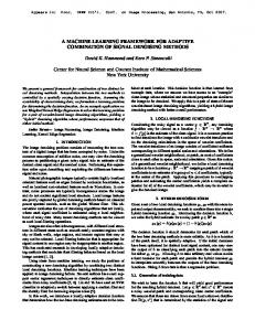
1.2

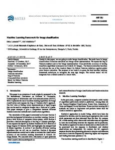
A schematic diagram of Temporal Enhanced Ultrasound (TeUS) data generation. A time series of a fixed point in an image frame, shown as a red dot, is analyzed over a sequence of ultrasound frames to determine tissue characteristics. . . . . . A schematic diagram of TeUS-based workflow for prostate biopsy. . . . . . . . . . . . . . . . . . . . . . . . . . . . . . . .

UroNav MR/US fusion system: The identified mp-MRI lesions were delineated on the T2-weighted MR image as the biopsy targets. The target location is shown by the green point along the projected needle path in the ultrasound image. . . . . . 2.2 Statistics of histopathology and MR readings in our TeUS dataset: Histopathology reports include the Gleason Score (GS) and the percentage distribution of prostate cancer. The MR scores were grouped into three descriptors of “low”, “moderate” and “high”, and referred to as the MR suspicious level assigned to the area. . . . . . . . . . . . . . . . . . . . . . . . 2.3 Example of distance maps and their corresponding B-mode and RF frames: (a) RF distance map, (b) RF frame, (c) B-mode distance map, (d) B-mode frame. The dark blue is showing the target location and the color spectrum from blue to yellow is showing farther distance from the target. . . . . . 2.4 Preprocessing and ROI selection: the target region is divided to 80 ROIs of size 0.5 mm×0.5 mm and then a sliding window is used for the data augmentation. . . . . . . . . . . . . . . .

8 12

2.1

3.1

An illustration of a Restricted Boltzmann Machine (RBM): RBM consists of a layer of binary stochastic visible units v, connected to a layer of stochastic hidden units h by symmetrically weighted connections W. . . . . . . . . . . . . . . . . .

23

24

26

26

31

xv

List of Figures 3.2

3.3 3.4

3.5

3.6

3.7

3.8

An illustration of the proposed method for prostate cancer detection. Our DBN has a layer of real-valued visible units of dimension F = 50 and four hidden layers with 100, 50 and 6 hidden units. The red box contains the pre-trained DBN, and the blue box containing one neuron is added for the fine-tuning step. The latent features are the output of the last layer of DBN. . . . . . . . . . . . . . . . . . . . . . . . . . . . . . . . An illustration of the proposed feature visualization method. Cancer probability maps overlaid on B-mode ultrasound image, along with the projected needle path in the temporal ultrasound data and centered on the target. The ROIs for which the cancer likelihood is more than 70% are colored in red, otherwise they are colored in blue. The green boundary shows the segmented prostate in MRI projected in TRUS coordinates, dashed line shows needle path and the arrow pointer shows the target: (a) Correctly identified benign core; (b) Correctly identified the cancerous core. . . . . . . . . . . . Investigation of the effect of tumor size on accuracy. We obtained the average AUC of 0.77 for cores with MR-tumorsize smaller than 1.5 cm, and the average AUC of 0.93 for cores with MR-tumor-size larger than 2 cm. . . . . . . . . . . Differences of distributions between cancerous and benign tissue back projected in the input neurons: (a) corresponds to the first neuron in the third hidden layer; (b) corresponds to the sixth neuron in the third hidden layer. Results are shown in the frequency range of temporal ultrasound data analyzed in this section. It is clear that frequencies between 0 − 2 Hz provide the most discriminative features for distinguishing cancerous and benign tissue. . . . . . . . . . . . . . . . . . . . Overview of the proposed method. We use two layers of RNNs with LSTM cells to model the temporal information in a sequence of TeUS data. x(i) = (x1 , , ..., xT ), T = 100 is showing the ith sequence data and xt is indicating the tth time step. . . . . . . . . . . . . . . . . . . . . . . . . . . . . . . . . Comparison between optimizer performance for different RNN cells: Each curve corresponds to an RNN network structure with two hidden layers, batch size of 128 with the dropout rate of 0.2 and regularization term of 0.0001. . . . . . . . . .

35 37

42

42

43

45

51

xvi

List of Figures 3.9

Learning curves of different RNN cells using the optimum hyper-parameters in our search space. All of the models use the RMSprop optimizer and converge after 65±7 epochs. . . . 3.10 Cancer likelihood maps overlaid on B-mode ultrasound images, along with the projected needle path in the TeUS data, and centered on the target. Red indicates predicted labels as cancer, and blue indicates predicted benign regions. The boundary of the segmented prostate in MRI is overlaid on TRUS data. The arrow points to the target location. The top row shows the result of LSTM and the bottom row shows the result of spectral analysis [11] for benign targets (a), and cancer targets (b) and (c). . . . . . . . . . . . . . . . . . . . . 3.11 Sequence Length effect: The most discriminative features for detection of prostate cancer can be learned from a fraction of the full TeUS time series. . . . . . . . . . . . . . . . . . . . . 4.1 4.2 4.3

4.4

4.5

4.6

53

56

57

An illustration of the proposed cancer grading approach using spectral analysis of TeUS. . . . . . . . . . . . . . . . . . . . . An illustration of the proposed GMM initialization method. . Cancer likelihood maps overlaid on B-mode US image, along with the projected needle path in the TeUS data and centered on the target. The ROIs for which we detect as Gleason grade of 4 and 3 are colored in red and yellow, respectively. The non-cancerous ROIs are colored as blue. The red boundary shows the segmented prostate in MRI projected in TRUS coordinates and the arrow pointer shows the target. . . . . . Target location and distribution of biopsies in the test data. Light and dark gray indicate central and peripheral zones, respectively. The pie charts show the number of cores and their histopathology. The size of the chart is proportional to the number of biopsies (in the range from 1 to 25), and the colors dark red, light red and blue refer to cores with GS≥ 4 + 3, GS≤ 3 + 4 and benign pathology, respectively. The top, middle, and bottom rows depict histopathology results, TeUS prediction, and integration of TeUS and MRI, respectively. Model performance for prostate cancer grading using spectral analysis of TeUS and distribution learning in the test dataset and permutation set. . . . . . . . . . . . . . . . . . . . . . . . Model performance for different sizes of training dataset using spectral analysis of TeUS and distribution learning. . . . . . .

63 65

67

69

70 70

xvii

List of Figures 4.7

4.8

4.9

4.10 4.11

Model performance versus the number of features that we used to generate the final model: (a) For all of the cores; (b) for cores with MR-tumor-size≥ 2.0 cm. Decreasing the number of features improves the model performance. . . . . . . . . . Illustration of noisy and not finely annotated ground-truth label. The exact location of the cancerous ROI in the core, the ratio of the different Gleason grade, and the exact location of the Gleason grades are unknown and noisy. The bottom vectors show one of the possible multi-label binarization approaches. . . . . . . . . . . . . . . . . . . . . . . . . . . . . . Overview of the second stage in the proposed method: the goal of this stage is to assign a pathological score to a sample. To mitigate the problem of imperfect and noisy labels, we embed the length of cancer in the ground-truth probability vector as a soft label. . . . . . . . . . . . . . . . . . . . . . . . Scatter plot of the reported tumor in core length in histopathology vs. the predicted tumor in core length. . . . . . . . . . . (a) Cancer likelihood maps overlaid on B-mode US image, along with the projected needle path in the TeUS data (GS ≥ 4 + 3) and centered on the target. The ROIs of size 0.5 × 0.5 mm×mm for which we detect the Gleason grade of 4 and 3 are colored in red and yellow, respectively. The non-cancerous ROIs are colored as blue. (b) The red boundary shows the segmented prostate in MRI projected in TRUS coordinates and the arrow pointer shows the target.[blue=low uncertainty, red=high uncertainty] . . . . . . . . . . . . . . . . . . . . . .

An illustration of the proposed approach for domain adaptation between RF and B-mode time series data in TeUS framework. . . . . . . . . . . . . . . . . . . . . . . . . . . . . 5.2 Learning curve for DBN training based on the cross-entropy: (a) for first hidden layer size. (b) for different learning rates (LR). (c) for different mini-batch size (BS). In a coarse search for the meta-parameters we achieved the lowest cross entropy loss with n = 44, LR = 0.2, and BS = 10. . . . . . . . . . . . 5.3 Distribution shift from B-mode to RF for the top three features before (top row) and after (bottom row) the shared deep network. The proposed domain adaptation method can effectively align features and reduce the distribution shift in common learned feature space. . . . . . . . . . . . . . . . . .

71

72

74 79

80

5.1

85

90

91 xviii

List of Figures 5.4

Influence of labeled dataset size in classification accuracy: performance of the method measured by AUC, accuracy, sensitivity and specificity in the k-fold cross-validation setting for (a) TeUS RF data and (b) TeUS B-mode data. . . . . . . . . 93 5.5 The comparative performance of the proposed method meaS sured by AUC over the baselines for Dtest . . . . . . . . . . . 95 5.6 Cancer probability maps overlaid on B-mode US image, along with the projected needle path in the temporal US data and centered on the target. The ROIs for which the cancer likelihood is more than 50% are colored in red, otherwise they are colored as blue. The red boundary shows the segmented prostate in MRI projected in TRUS coordinates, dashed line shows needle path and the arrow pointer shows the target: (a)-(c) Correctly identified cancerous core using RF time series data; (b)-(d) Correctly identified cancerous core using B-mode time series data. . . . . . . . . . . . . . . . . . . . . . . . . . 96 5.7 Guidance interface implemented as part of a 3D Slicer module: cancer likelihood map is overlaid on B-mode ultrasound images. Red indicates predicted labels as cancer, and blue indicates predicted benign regions. The boundary of the segmented prostate is shown with white and the green circle is centered around the target location which is shown in the green dot. . 100 6.1 6.2 6.3

An illustration of the proposed feature visualization method. Pathology mimicking simulations framework. . . . . . . . . . ROI selection and nuclei-based scatterer generation process: (a) Sample of histopathology slide [70], where the red boundary depicts the cancer area; (b) digitized slide overlaid on the histopathology slide, where green and red areas represent the benign and cancer regions, respectively. The selected ROIs are shown by black squares; (c) extracted nuclei positions in the selected ROIs; left: a cancer region, right: a benign region; (d) the extracted positions of nuclei from each ROI is embedded in an FEM model. . . . . . . . . . . . . . . . . . . . . . . . . 6.4 (a) A sample whole-mount histopathology slide of the prostate. Different regions of cancer and benign tissue are shown in the pathology slide. (b) The corresponding simulated B-mode ultrasound image. . . . . . . . . . . . . . . . . . . . . . . . .

107 108

109

110

xix

List of Figures 6.5

(a) Differences of distributions between cancerous tissues with Gleason patterns 3 and 4 as well as benign tissues back projected in the input neurons corresponds to the first neuron in the third hidden layer; (b) Spectral difference of the simulated TeUS in benign and different cancer tissues. . . . . . . . . . . 111 6.6 (a) Distribution of the power spectrum in the frequency spectrum of simulated TeUS data at the excitation frequency, (b) Distribution of the power spectrum in the frequency spectrum of simulated TeUS data at the first harmonic of the excitation frequency. . . . . . . . . . . . . . . . . . . . . . . . . . . . . . 112 B.1 Overview of the biopsy guidance system. The three steps in the guidance workflow are volume acquisition, classification and guidance. A client-server approach allows for simultaneous and real-time execution of computationally expensive algorithms including TeUS data classification, and prostate boundary segmentation. . . . . . . . . . . . . . . . . . . . . . . . . . . . 144 B.2 The software system has a three-tiered architecture. Ovals represent processing elements while arrows show the direction of data flow. In the US machine layer, PLUS is responsible for US data acquisition and communicates with the TeUSclient via the OpenIGTLink protocol. The TeUS client layer includes TeUS guidance, an extension module within the 3D Slicer framework. The TeUS-server layer is responsible for the simultaneous and real-time execution of computationally expensive algorithms and communicates with TeUS-client via the OpenIGTLink protocol. . . . . . . . . . . . . . . . . . . . 145

xx

Glossary AUC Area Under the ROC Curve B-mode Brightness Mode CD Contrastive Divergence CNNs Convolutional Neural Networks DBN Deep Belief Networks DNN Deep Neural Networks DFT Discrete Fourier Transform DRE Digital Rectal Exam DCE Dynamic Contrast Enhanced DWI Diffusion Weighted Imaging EM ElectroMagnetically GMM Gaussian Mixture Model GPU Graphics Processing Unit GRU Gated Recurrent Unit GS Gleason Score HMMs Hidden Markov Models FEM Finite Element Model FWHM Full Width at Half Maximum ICA Independent Component Analysis KL Kullbac–Leibler xxi

Glossary LSTM Long Short-Term Memory MRE Magnetic Resonance Elastography MRI Magnetic Resonance Imaging MSE Mean Squared Error mp-MRI multi-parametric MRI NCI National Cancer Institute NIH National Institutes of Health PCa Prostate Cancer PCA Principal Component Analysis PSA Prostate Specific Antigen PSF Point Spread Function RBF Radial Basis Function RBM Restricted Boltzmann Machine RF Radio Frequency RFE Recursive Feature Elimination RNNs Recurrent Neural Networks ROC Receiver Operating Characteristic ROI Region of Interest SEER Surveillance, Epidemiology, and End Results SDM Subspace Disagreement Measure SGD Stochastic Gradient Descent SVM Support Vector Machine TeUS Temporal Enhanced Ultrasound TRUS Transrectal Ultrasound US Ultrasound xxii

Acknowledgements First and foremost, I would like to express my sincerest gratitude to Prof. Purang Abolmaesumi, my advisor, for the opportunities you gave to me. Thank you for your trust, patience and invaluable support that opened this chapter of my life. Thanks for the generosity, advice and friendship you offered me throughout my experience at UBC. I am very grateful for being associated with Prof. Parvin Mousavi, whose insightful advices helped me throughout the course of this endeavor. Her patience, dedication, mentorship and sincere advice in every single step of the thesis have been truly crucial. Thanks for being always supportive and enthusiastic. I would like to thank supervisory committee Professors Salcudean and Rohling for their valuable comments and advices. I would like to thank the Natural Sciences and Engineering Research Council of Canada (NSERC), the Canadian Institutes of Health Research (CIHR), Philips Research North America, and UBC for funding this work.

xxiii

Dedication I dedicate this to my parents who left fingerprints of grace on my life; my family without whom none of my success would be possible, you are my wings to fly.

xxiv

Chapter 1

Introduction If I have seen farther it is by standing on the shoulders of Giants. — Sir Isaac Newton

1.1

Prostate Cancer Diagnosis

Prostate Cancer (PCa) is a significant public health issue, and approximately 14% of men will be diagnosed with this disease at some point during their lifetime 1 . According to the American and Canadian Cancer Societies, prostate cancer accounts for 24% of all new cancer cases and results in 33,600 deaths per year in North America 2 . If diagnosed in the early stages, it can be managed with a long-term disease-free survival rate above 90%; even if it is identified later, interventions can be used to increase the life expectancy of patients. The prostate cancer-related death rate has declined significantly (almost 4% per annum) between 2001 and 2009 due to improved testing and better treatment options. The majority of the cases diagnosed today are the early-stage disease, where several treatment options are available, including surgery, brachytherapy, thermal ablation, external beam therapy, and active surveillance. Early detection and accurate staging of prostate cancer are essential to the selection of optimal treatment options. Hence, reducing the disease-associated morbidity and mortality [134]. Currently, prostate cancer detection is carried out by a combination of Digital Rectal Exam (DRE), measurement of the Prostate Specific Antigen (PSA) level, and histological assessment of biopsy samples. DRE is the most common and least expensive way to screen for prostate cancer. However, DRE is only effective for detecting late-stage prostate cancer in the peripheral zone of the gland, and any abnormalities located in other prostate zones cannot be felt. The PSA test measures the blood level of 1

National Cancer Institute (NCI): Surveillance, Epidemiology, and End Results (SEER) Cancer Statistics Review 2 Canadian cancer society: http://www.cancer.ca/, and American cancer society: http: //www.cancer.org/

1

1.1. Prostate Cancer Diagnosis PSA, a protein that is produced by the prostate gland and can be used as a biological marker for tumors. The elevated levels often indicate the presence of prostate cancer; however, it also increases by inflammation of the prostate gland (prostatitis), and when prostate enlarges with age (benign prostatic hyperplasia). Therefore, a reliable diagnosis cannot be performed by these two procedures [98]. The definite diagnosis of prostate cancer is core needle biopsy, under Transrectal Ultrasound (TRUS) guidance. The biopsy procedure entails systematic sampling of the prostate followed by histopathology examination of the sampled tissue. In systematic biopsy, up to 12 cores are taken from predefined anatomical locations. Conventional Ultrasound (US) imaging is not capable of distinguishing cancerous and normal tissue with high specificity and sensitivity. Therefore, the biopsy procedure is blind to intraprostatic pathology and can miss clinically significant disease. The sensitivity of conventional systematic biopsy under TRUS guidance, for detection of prostate cancer, has been reported to be as low as 40% [39, 56, 126, 134]. Significant improvement of TRUS-guided prostate cancer biopsy is required to decrease the rate of over-treatment for low-risk disease while preventing the under-treatment of high-risk cancer [89]. Several methods have been proposed to alleviate this issue by enabling patient-specific targeting to improve the detection rate of prostate cancer. Fusion of Magnetic Resonance Imaging (MRI) and TRUS-guided biopsy [41, 67, 122] as an emerging technology for patient-specific targeting is being gradually adopted and has shown significant potential for improved cancer yield [31, 119]. A meta-analysis of seven multi-parametric MRI (mp-MRI) studies with 526 patients shows specificity of 0.88 and sensitivity of 0.74, with negative predictive values ranging from 0.65 to 0.94 [37]. Although using mp-MRI in fusion biopsy has resulted in the best clinical results to date, recent studies suggest the high sensitivity of mp-MRI in the detection of prostate lesions but low specificity [3], hence, limiting its utility in detecting disease progression over time [145]. This approach has other limitations: (1) mp-MRI is often unfamiliar to the biopsying clinician; (2) the co-alignment of mp-MRI and TRUS is challenging [80, 81, 149]; and (3) mp-MRI is not specific for detecting prostate cancer with intermediate risk. Moreover, limited accessibility and high expense of MRI make an ultrasound-based prostate cancer detection system more preferable. The advantages of an ultrasound-based system are several folds: TRUS is already accepted as the standard prostate biopsy guidance tool; different ultrasound data and image acquisition techniques are simultaneously available on ultrasound machines, and ultrasound imaging is among the most accessible and least harmful medical imaging approaches. 2

1.2. Background

1.2 1.2.1

Background Ultrasound Techniques for Prostate Cancer Diagnosis

Since the early 1990s, there have been numerous efforts to improve ultrasoundbased tissue typing in the TRUS-guided biopsy. When tissue undergoes ultrasound imaging, returning echoes contain useful information for tissue typing. This information can be applied to discriminate among different tissues or to determine different structures of the same tissue due to diseases such as cancer. For prostate tissue typing, methods that not only distinguish prostate cancer but also provide information on its grade, have the potential to improve the management of cancer and its treatment while preventing over-diagnosis. In this section, we review ultrasound-based tissue typing approaches and their application in prostate cancer diagnosis. Major ultrasound-based tissue typing methods for prostate cancer characterization include texture-based and spectral analysis of ultrasound data, elastography, Doppler, and ultrasound time series analysis. 1.2.1.1

Texture-based and Spectral Analysis

The intensity information in Brightness Mode (B-mode) ultrasound images can be used to differentiate among various tissue types [112, 126]. For texture-based tissue characterization, the image is divided into windows called a Region of Interest (ROI). ROI sizes between 0.1 cm × cm and 1.45 cm × cm have been reported in the literature [112]. Texture-based methods analyze the first and second order statistics of the gray levels of the B-mode images which form a set of features for texture characterization. The firstorder statistics include the mean, standard deviation, skewness and kurtosis of the gray level in each ROI. Moreover, the speckle signal-to-noise ratio, maximum and minimum, and the Full Width at Half Maximum (FWHM) of ROIs have been found useful for prostate tissue typing [140]. These features are sensitive to imaging parameters of ultrasound scanners and dissimilar acoustical properties for tissues with the same pathology have been observed [112]. Probability distribution models (e.g., Rayleigh, Rice, and Nakagami) fitted to the estimated histogram of B-mode image intensities have also been shown to provide useful clinical information for tissue characterization [30, 152]. Tsuni et al. [151] showed that the B-mode image would be affected by the system settings and user operations. They suggested that the Nakagami parametric image provides a comparatively consistent image result when different diagnosticians use different dynamic ranges and system gains. Their 3

1.2. Background result indicated a better performance of this distribution model compared to other models for prostate cancer diagnostics. Although statistical texturebased features extracted from ultrasound B-mode image are important for tissue typing, they have not been used alone [126]. The combination of texture-based features with features extracted from other ultrasound techniques [106] and other modalities [7] have been shown to be effective. Second-order statistical features have been introduced to overcome these limitations. These features are related to the spatial properties of the image and are extracted from the co-occurrence and auto-correlation matrices of B-mode image [17, 129, 140, 141]. Although statistical texture-based features extracted from B-mode and envelope detected signals are necessary for tissue typing, they are usually combined with features extracted from other methods for tissue characterization [112]. Combining texture-based and clinical features such as location and shape of the hypo-echoic region can be a promising way to detect prostate cancer. It has been shown that cancerous tissues can be detected with high specificity (about 90-95%) and high sensitivity (about 92-96%) applying the combination of the features [59]. The main shortcomings of texture-based methods are their high dependency on imaging settings of the ultrasound scanner, signal attenuation, dropout, and shadowing. Some of the tissue-dependent features can only be extracted from Radio Frequency (RF) echo signals before they go through the nonlinear process of envelope detection for B-mode image generation [44, 112, 127]. During the past decades, spectral analysis of RF echo signals constituting a single ultrasound image has been used to improve prostate cancer diagnosis. One of the earliest attempts at using spectral analysis of ultrasound has been by developing an analog filter to break the bandwidth of backscattered ultrasound into three bands [64]. A few years later, Lizzi and Feleppa as the pioneers of spectral analysis of ultrasound signals developed a theoretical framework for the spectral analysis of ultrasound [97]. In this framework, they proposed a method for calibration of the spectrum to account for systemdependent effects. Lizzi et al. categorized tissue structures theoretically based on the spectral properties of ultrasound backscattered signals [96]. Spectral features extracted from the power spectrum of the signals have been used to distinguish between normal and cancerous tissues in the prostate by Feleppa et al. [42, 43]. There are models which represent the relation between spectral features and tissue microstructure theoretically [96]. However, in practice, local spectral noise, and system-dependent effects are challenges for using these techniques [96, 123]. Recently, histoscanning [100, 101], a commercial software that uses features of a single RF frame, has been applied 4

1.2. Background to characterize prostate cancer. Studies have reported an average sensitivity of 60% and specificity of 66% for 146 patients using this approach [101]. In Section 1.2.2, we will further explore this category of techniques in more details from a machine learning perspective. 1.2.1.2

Elastography

Soft tissues tend to exhibit higher deformation than stiffer areas when compression is applied. Elastography is an ultrasound imaging approach that aims to capture tissue stiffness. Since cancerous regions of the tissue are usually stiffer than benign regions, elastography can be helpful for prostate cancer characterization [55, 124]. The quasi-static methods and dynamic methods are two main ultrasound elastography categories. Quasi-static ultrasound elastography or strain elastography of the prostate is based on the analysis of the deformation generated by a static compression of the tissue using TRUS. Krouskop et al. [88] analyzed the prostate tissue samples to evaluate the elastic properties of the tissue specimens. These properties were also used by Konig et al. [85] for image-guided biopsy of the prostate in a group of 404 patients. In this study, 84% of positive cancer patients were correctly identified [85]. Improvement in biopsy guidance [25, 79, 85, 130] and prostate cancer identification [25, 34, 38, 52, 139] are reported in the literature. However, some well-designed studies did not confirm such results [130, 152]. The main limitations of strain elastography include lack of uniform compression over the entire gland, dependency on the operator, penetration issues in large glands, and artifacts due to slippage of the compression plane that can occur in up to 32% of images [25, 34]. A water-filled balloon may be placed between the probe and the rectal wall to improve the homogeneity of the deformation and reduce the artifacts [4]. In dynamic methods, a time-varying force is applied to the tissue; it can be either a short transient mechanical force or an oscillatory force with a fixed frequency [49, 65]. Several dynamic methods have been proposed including vibro-elastography [2, 66, 99, 138], Acoustic Radiation Force Impulsion (ARFI) [121], and shear wave elastography [23, 24]. Vibro-elastography is operator independent and can be used to estimate the stiffness of the tissue using TRUS [2, 66, 99, 138]. Shear wave elastography is the most recent elastography technique, which is based on the measurement of low-frequency shear wave velocity propagating through the tissue [32, 49]. While the specificity of shear wave elastography has been reported to be as high as 91%, the reported sensitivity can be relatively low (63%) [78, 120]. Other 5

1.2. Background limitations of shear wave elastography include slow frame rate, limited size of the ROI, delay in image stabilization for each acquisition plane and signal attenuation in enlarged prostates, making the evaluation of the anterior transitional zone difficult or impossible [32]. Most of the current clinical elastography systems are only capable of producing an image that visualizes a single tissue physical parameter, such as stiffness or viscosity, while cancerous tissues are complex and non-uniform and cannot be characterized using only one parameter [7, 55, 106]. To address this limitation, more recently, multi-parametric elastography ultrasound and its combination with multi-parametric MRI have been considered. Mohareri et al. [106] showed the potential of multi-parametric quantitative vibro-elastography in prostate cancer detection for the first time in a clinical study including 10 patients. Ashab et al. [7] also combined multiparametric MRI with multi-parametric ultrasound, including B-mode and vibro-elastography images. In a study including 36 whole mount histology slides, they examined the potential improvement in cancer detection. The idea of capturing tissue stiffness has been extended to MRI as well, and has been explored as Magnetic Resonance Elastography (MRE) technique [136, 137] for detection of tissue abnormalities. In MRE, an external mechanical excitation is applied to the tissue of interest to induce tissue vibrations and it has been shown to be of value in MRI tissue characterization. Despite major advancement in the elastography technology, all these approaches are subject to the same intrinsic limitations: “not all cancers are stiff, and all stiff lesions are not cancerous” [32, 137]. 1.2.1.3

Doppler Imaging

Doppler imaging is an alternative ultrasound-based technique for detection of pathologic conditions. Doppler-based cancer detection methods take advantage of the neovascularization phenomenon in cancerous tissues; changes in cellular metabolism associated with the development of cancer leads to an increase in blood supply to cancer lesions and therefore to neovascularization in the malignant area [57]. A fundamental problem in Doppler-based cancer detection is that blood is a much weaker scatterer of the ultrasound than the surrounding tissue. Therefore, a considerable frequency shift is required to separate a Doppler signal from the background signal. This challenge normally limits Doppler studies to larger vessels with high blood velocity [112]. Moreover, neovascularization related to prostate cancer is usually at the microvascular level which restricts the applicability of Doppler analysis in prostate cancer detection [114]. Today, color flow images, power Doppler 6

1.2. Background imaging, and contrast-enhanced Doppler are all used for detecting prostate cancer and assisting biopsy procedure. Initial reports on the application of Doppler imaging for prostate studies date back to 1990 when the conventional color flow imaging was utilized for tissue characterization [159]. In a study including 39 subjects, Potdevin et al. [133] used mean of speed in colored pixels and speed-weighted pixel density to locally discriminate prostate cancer. A report from Arger et al. [6] showed that these two features were not substantially different between diverse pathologic tissues. In another study, Tang et al. [148] selected 54 patients with distinct cancer lesions on ultrasound images. They calculated the density of color pixels from Doppler images and used a t-test to analyze the relationship between the density ratio and malignancy. The obtained sensitivity of 91% in this study should be interpreted along with the large size of ROIs. In general, according to different studies, color Doppler imaging is useful for identifying prostate cancer, but targeted biopsy based on color Doppler imaging alone can miss many areas of cancer [120]. In a study of 120 patients, a biopsy regimen consisting of both sextant and color Dopplerdirected biopsies was more sensitive than sextant biopsies alone, but the improvement in cancer detection was minimal [86]. Nelson et al. [120] suggested that the area of hyper-vascularity must be large enough to stand out on the Doppler display. Thus, color Doppler may be more sensitive for detection of clinically significant, high-grade lesions. While contrast enhancing agents can increase the intensity of Doppler signal from the microvessels [25, 160], legal and technical difficulties have limited the application of such agents. 1.2.1.4

Ultrasound Time Series Analysis

Temporal Enhanced Ultrasound (TeUS) data is defined as the time series of RF echo signals obtained from a stationary position in a tissue without intentional motion of the transducer or the tissue [112] (Fig. 1.1). Since 2007, temporal enhanced ultrasound data has been explored using a machine learning framework to analyze subtle relative variations between various tissue types. It has been shown that features extracted from these variations, highly correlate with the underlying tissue structure [18]. A fundamental departure from prior methods is to display a likelihood map of the presence of cancer, based on machine learning, instead of using pre-defined thresholds for cancer detection. Machine learning eliminates the need for accurate thresholding of features to identify cancer. Moradi et al. utilized spectral features extracted from ultrasound RF time series signals to distinguish between different animal 7

1.2. Background

Figure 1.1: A schematic diagram of Temporal Enhanced Ultrasound (TeUS) data generation. A time series of a fixed point in an image frame, shown as a red dot, is analyzed over a sequence of ultrasound frames to determine tissue characteristics. tissue types [109]. The results of this study demonstrated that temporal ultrasound data are sensitive and specific for tissue typing. Moreover, in an ex vivo study, spectral time series features were applied to differentiate between healthy and cancer tissues in 35 human prostate specimens [108]. The results from this study showed that the features extracted from temporal enhanced ultrasound data are significantly more accurate and sensitive compared to the best texture-based and spectral features for detecting prostate cancer. In an in vivo experiment with six radical prostatectomy patients [73], and in a retrospective study with 158 patients undergoing fusion biopsy [11, 13, 82], accurate prostate cancer detection across grades and patients has been demonstrated. Evidence derived from the experiments to-date suggests that both tissue-related and ultrasound signal-related factors lead to tissue typing information in temporal enhanced ultrasound data. These include the cellular structure of the tissue [109] and the thermal properties of the tissue at micro-scale [36]. For the work presented in this dissertation, TeUS is the imaging modality used for data collection in prostate cancer patients. 8

1.2. Background

1.2.2

Machine Learning Approaches

From the computer-aided diagnosis point of view, prostate cancer detection using ultrasound imaging, can be automated as a classification or a clustering task. Over the past decades, machine learning methods are employed to automate the process of tissue typing using handcrafted features, and more recently, to automatically derive features that optimally represent the data based on tissue types. In this section, I focus the discussion on these two major approaches for deploying machine learning techniques in prostate cancer diagnosis. 1.2.2.1

Feature Generation and Classification

Previously, manually engineered feature representations extracted from ultrasound data [72, 73, 76] have been used with shallow discriminant models such as linear regression models [42–44], k-Nearest Neighbours (k-NN) classifier [98], support vector machines (SVM) [45, 108], random forests [51, 154], Bayesian classifiers [113] and multi-layer feed-forward perceptron networks [44, 109], to differentiate tissue types [112]. Feleppa et al. [42, 43, 45] extracted the spectral-features for tissue typing in prostate cancer from a line fitted to the power spectrum of a single frame of RF echo signal obtained by sonicating the tissue of interest. In this approach, after using Fourier transform to map the RF signals into the spectral domain, they used a linear regression model to explain the relationship between frequency and amplitude in the power spectrum. The extracted features from the regression model, such as intercept and slope were used for differentiation between tissue types. Llobet et al. proposed the adoption of a k-NN classifier to detect cancerous regions in transrectal ultrasound B-mode images of the prostate [98] where they utilized texturebased feature extracted from the ultrasound images to train their classifier. Mohareri et al. [106] proposed a novel set of features that obtained from vibro-elastography to classify cancerous and normal tissue and compute a cancer probability map. These features include brightness, tissue strain, absolute value of tissue elasticity, relaxation time, and visco-elastic properties. They used a random forest classification framework to combine multi-parametric features and perform tissue characterization. In a leave-one-patient-out study including 10 patients, they achieved area under the receiver operating characteristic curve (AUC) of 0.8±0.01. Ashab et al. [7] proposed prostate tissue classification based on the combination of multi-parametric MRI and multi-parametric ultrasound which includes texture-based features from B-

9

1.2. Background mode images and vibro-elastography features. They used LASSO regression and Recursive Feature Elimination (RFE) for feature reduction and selection. Then, a weighted SVM was used for classification. In a study including 36 whole mount histology slides, they achieved an AUC of 0.81 for cancerous ROIs extracted from the peripheral zone of the prostates [7]. More recently, Imani et al. [73, 75] combined extracted features from discrete Fourier and Wavelet transforms of TeUS data and fractal dimension to characterize in vivo prostate tissue using SVMs. Imani et al. [75] used a joint Independent Component Analysis (ICA) algorithm to select the most informative and independent combination of features extracted from in vivo TeUS signal. Then, they trained an SVM classifier to differentiate between normal and cancer tissue. Ghavidel et al. [51] used spectral features of TeUS data and performed feature selection using random forests to classify lower grade prostate cancer from higher grades. Moradi et al. [109, 113] used fractal dimension with Bayesian classifiers and shallow feed-forward neural networks for ex vivo characterization of prostate tissue. Feleppa et al. [44] also used artificial neural networks to assess the performance of spectral features from RF echo signals collected during TRUS imaging of the prostate. 1.2.2.2

Hidden Markov Models

Hidden Markov models (HMMs) represent sequential data, especially time series, as stochastic processes through capturing repetitive patterns and motifs in the data. HMMs are based on probabilistic dependency and hence are well suited for describing time-varying sequences. Llobet et al. [98] proposed the use of HMMs for tissue characterization in TRUS images collected during prostate biopsies. They modeled the echo intensity values along the biopsy-needle path inside of the scanned tissue. The modeled sequences, in this case, are position-dependent rather than time-dependent. Most recently, analysis of TeUS in the temporal domain using probabilistic methods, such as HMMs, have shown significant promise [115, 118]. Nahlawi et al. [116–118] used HMMs to model the temporal information of TeUS data for prostate cancer detection. In a limited clinical study including 14 subjects, they identified cancerous regions with an accuracy of 85%. Their results also indicate the importance of order in the characterization of tissue malignancy from TeUS data [115].

10

1.3. Proposed Solution 1.2.2.3

Deep Learning Approaches

Deep learning algorithms are probabilistic models (networks) composed of many layers that transform input data (e.g., images) to outputs (e.g., disease present/absent) while learning increasingly higher level features [61, 95]. In the computer-aided diagnosis literature, Deep Neural Networks (DNN) [63, 95] have been recently established as a powerful machine learning paradigm. The main advantage of DNNs is their ability to discover informative representation of data which contributes to feature engineering originally performed solely by human experts. Our group previously examined Convolutional Neural Networks (CNNs) to combine temporal and spatial information from TeUS data to detect high-risk prostate cancer. Imani et al. [74] used a machine learning framework consisting of the weighted combination of two CNNs. One network takes the information in the temporal sequence as input while the other network uses the spatial arrangement of the ultrasound data. Then, they use the fusion of mp-MRI and TeUS for characterization of higher grade prostate cancer. In a leave-one-patient-out evaluation including 14 patients, they achieved the Area Under the ROC Curve (AUC) of 0.86 for cancerous regions with GS≥3+3, and AUC of 0.89 for those with GS≥3+4. Besides being computationally expensive, large-scale data is required for effective deep learning and to ensure proper generalization. Further, the difficulty in explaining the operation of deep neural networks has led to imperceptive and repetitive, yet successful use of deep learning methods as a black-box in many areas. The focus of this thesis is on probabilistic modeling of spectral and temporal aspect of TeUS data using Deep Belief Networks (DBN) [62] and Recurrent Neural Networks (RNNs) [50], respectively. In addition, methodologies are devised to interpret the internal representations learned by deep models to derive insights about tissue dependent features residing in TeUS.

1.3

Proposed Solution

Despite many years of research to improve prostate cancer diagnosis, conventional ultrasound-guided biopsy has low sensitivity, leading to significant rates of under-treatment and over-treatment. Augmentation the biopsy process with ultrasound-based tissue typing techniques that analyze the spectrum and texture of TRUS, or measure mechanical properties of tissue in response to external excitation is useful. However, individual methods have not shown success in multi-center clinical studies, as it is proven difficult to establish a cancer-specific tissue property consistent across the population [102]. 11

1.3. Proposed Solution

T2

PCa Suspect

Ktrans

Multiparametric MRI

Pre-Procedure Intra-Procedure

Systematic Biopsy

Fusion Biopsy

Biopsy Procedure

US Targeted Biopsy

Transrectal US

MR-TRUS fusion

Proposed Decision Support Model

Temporal US data

Figure 1.2: A schematic diagram of TeUS-based workflow for prostate biopsy. The focus of this thesis is to advance prostate cancer diagnosis through the development of a deep learning solution for real-time analysis of temporal enhanced ultrasound image. The proposed solution will be trained to automatically analyze backscattered ultrasound signals from the tissue over a multitude of TRUS frames and extract tissue-dependent features to discriminate between different cancer grades. The proposed solution can be deployed as a decision support model for patient-specific targeting during biopsy; it can display cancer likelihood maps on B-mode ultrasound images, in real-time, to indicate the presence of cancer. Moreover, its fusion with MRI, where available, can be used to improve biopsy targeting (Figure 1.2). A fundamental assumption in previous models for TeUS is the availability of RF data in imaging equipment; however, RF is not available on all commercial US scanners and is usually only provided for research purposes. To overcome the challenge of accessibility of RF data, in the TeUS machine learning framework, we propose to use a transfer learning method [131] to transfer knowledge between RF and B-mode data within an ultrasound scanner. Transfer learning is a method that can compensate for the diversity between datasets by learning from a source dataset (RF time series data) and applying the knowledge to a target dataset (B-mode time series data). This approach exploits the common information between the two domains. Common elements between two data domains can be features of the data or parameters of the models that are built using the data [131]. Deep learning methods, such as DBN, have an essential characteristic that makes them well suited for transfer learning: they can identify abstract features that perform well generalizing across various domains [21, 53]. The model is generated from RF or B-mode TeUS before the biopsy procedure and we can 12

1.3. Proposed Solution use the generated model to extract real-time tissue-dependent information from the temporal enhanced ultrasound signals. The proposed solution leverages the standard TRUS imaging pipeline (Figure 1.2), hence does not require modifications to the established clinical workflow. We expect that this technology provides a versatile cross-institutional solution for accurate detection of prostate cancer and patient-specific biopsy targeting.

1.3.1

Objectives

As explained before, the extensive heterogeneity in morphology and pathology of prostate adenocarcinoma are challenging factors in obtaining an accurate diagnosis using different imaging modalities. Providing tissue-specific information during TRUS-guided biopsies can assist with targeting regions with high probability of being cancerous. The analysis of TeUS reveals a difference in response between benign and malignant tissues as reported by several previous studies. The objectives of this thesis are: • Objective 1. Detection of prostate cancer using TeUS data. The first step towards improvement of TRUS-based targeted biopsy is to develop an accurate ultrasound-based tissue typing method. Deep learning techniques are proposed to automatically extract tissue-dependent features from in vivo temporal enhanced ultrasound data. These abstract high-level features can be used to distinguish between different prostate tissue types. • Objective 2. Detection of high-grade prostate cancer using TeUS data. The second step towards the improvement of the TRUSbased targeted biopsy is to develop a tissue typing method that can differentiate among grades of the disease and its extent. The ubiquity of noise is an important issue for building computer-aided diagnosis models for prostate cancer biopsy guidance where histopathology data is sparse and not finely annotated. A solution is proposed to alleviate this challenge as a part of the TeUS-based prostate cancer biopsy guidance method. • Objective 3. Development of a real-time TeUS-based decision model, and enabling its clinical deployment. Following successful diagnosis and grading of prostate cancer using deep models, the third objective is to enable its clinical deployment as a tool for improving detection of clinically significant prostate cancer in fusion biopsies. Towards this goal, the ability to remove TeUS spectrum 13

1.3. Proposed Solution analysis as a preprocessing step is studied by analyzing data directly in the time domain using Recurrent Neural Networks (RNNs). This can help reduce computation time and accelerate cancer likelihood map generation. Due to limited access to raw ultrasound data, transfer learning is devised to generate comparable performance using B-mode images. Real-time implementation of TeUS-based decision model and its evaluation through retrospective data is another step in realizing this objective. Finally, understanding the physical interaction of TeUS data with tissue is not only of theoretical benefit, but can help with practical decisions in building a decision model.

1.3.2

Contributions

This thesis develops, deploys and evaluates a deep learning framework that uses temporal enhanced ultrasound data to output accurate prostate cancer likelihood maps, overlaid on real-time TRUS images. The proposed solution encapsulates the variability associated with the access of raw ultrasound signals in commercial scanners, and can provide complementary information about the grade and extent of prostate cancer. In the course of achieving the objectives, the following contributions were made: 1. Probabilistic modeling of spectral information in temporal enhanced ultrasound: – An automatic feature selection framework is proposed based on DBN for spectral analysis of temporal enhanced ultrasound signals from prostate tissue. – A statistically significant improvement in the accuracy of prostate cancer detection is demonstrated compared to previously published studies using spectral features of TeUS signals [74, 76]. – To determine the characteristics of non-cancerous and cancerous cores in TeUS data and their correlation with learned features, a feature visualization approach is developed. This approach is used to identify the most discriminating frequency components of the time series as learned by the classifier. 2. Probabilistic modeling of temporal aspects of TeUS: – TeUS data is extensively and explicitly analyzed in temporal domain using time-dependent probabilistic deep networks for the first time. 14

1.3. Proposed Solution – Results indicated that RNN can identify temporal patterns in data that may not be readily observable in spectral domain, leading to significant improvements in detection of prostate cancer. – Algorithms are developed for in-depth analysis and visualization of high-level latent features of LSTM-based RNN. – A transformational finding, achieved through this analysis, is that the most discriminating features for detection of prostate cancer can be learned from a fraction of the full TeUS time series. Specifically, in this data, less than 50 ultrasound frames were required to build models that accurately detect prostate cancer. This information can be used to optimize TeUS data acquisition for clinical translation. 3. Classifying prostate cancer grade using probabilistic modeling of spectral aspects of TeUS data: – A novel approach for grading and detection of high-grade prostate cancer using spectral analysis of TeUS with DBN is proposed. – This approach could successfully differentiate among aggressive prostate cancer (GS≥4+3), clinically less significant prostate cancer (GS≤3+4), and non-cancerous prostate tissues. 4. Classifying prostate cancer grade and its extent based on temporal modeling of TeUS data: – A novel approach is devised for grading and detection of highgrade prostate cancer using temporal analysis of TeUS with RNN. By encapsulating proposed ground-truth probability vectors, this solution can also precisely estimate cancer length in biopsy cores. – The accuracy of tissue characterization is statistically significantly improved as compared to previously published studies [10, 12, 76]. – A novel strategy is proposed for depiction of patient-specific colormaps for biopsy guidance including the estimated model uncertainty. 5. Development of real-time TeUS-based decision model: – A transfer-learning approach is developed to address limited access to raw ultrasound data on commercial scanners, and scanner differences in multi-center settings. 15

1.3. Proposed Solution – Near real-time augmentation of live standard 2D ultrasound images with cancer likelihood maps generated from the models is implemented. – The viability of using B-mode TeUS for cancer detection is demonstrated using retrospective data. The initial assessment indicates that the solution is capable of providing guidance information for prostate biopsy procedures. 6. Investigation of the physical phenomena underlying TeUS: – A method for visualization and interpretation of the learned features from TeUS data is presented. – Evidence derived from feature visualization points to low-frequency components of TeUS as the most informative features for tissue classification. These components potentially represent the effect of pulsation on prostate tissue microstructure in form of microvibrations. – The effect of micro-vibration is simulated using a medium with preset elasticity and scatterer locations extracted from 14 wholemount digital histopathology slides. – Results demonstrated that the distribution and micro-vibration of scatterers could lead to tissue typing information in TeUS. This finding is a major breakthrough in understanding and technical formulation of TeUS after a decade. One million patients in North America undergo prostate biopsy annually; 70% of 10 core biopsies return negative while up to 34% of the positive yield are under-graded. The mp-MRI, as the state-of-the-art imaging technique for prostate cancer detection, has low accuracy in identifying cancer with intermediate-risk or low volume [89], and has a high rate of false positives, leading to a significant number of negative cores in current fusion biopsies [132, 144]. Cancer likelihood maps displayed by the proposed solution can help systematic biopsy by improving the cancer yield and decreasing the number of unnecessary biopsies. They also benefit fusion biopsy as they can compensate for inaccurate co-alignment of mp-MRI, improving the accuracy of mp-MRI especially for intermediate risk cancer. Innovative and transparent deep learning solutions will allow the technology to work across institutions without bias towards the image settings, equipment or patient pool in one setting. In the long term, this technology can benefit patients by enabling periodic examination of those under active surveillance by this technology alone. 16

1.3. Proposed Solution All men who undergo prostate biopsy can take advantage of the proposed technology by improving early detection of prostate cancer and decreasing the number of unnecessary biopsies. Further, the proposed solution can benefit patients by enabling periodic, affordable, widely available and minimallyinvasive examination of those under active surveillance, where it is critical to detect clinically significant prostate cancer early with a minimal number of biopsies.

1.3.3

Thesis Outline

The rest of this thesis is subdivided into six chapters as outlined below: Chapter 2: Temporal Enhanced Ultrasound Data This chapter describes the TeUS data acquired and analyzed in this thesis. It explains the clinical process of data acquisition and establishing ground truth prior to data analysis. Time-domain and spectral-domain representations of TeUS signals are also described. Chapter 3: Diagnosis of Prostate Cancer Using TeUS For accurate diagnosis of prostate cancer, in this chapter, both the spectral and temporal aspect of TeUS data are analyzed. The focus of the chapter is to distinguish two main categories of the tissues (i.e., cancer and benign) which can be modeled as a binary classification task: – Spectral analysis of TeUS using DBN: In this section, a deep learning approach is proposed to automatically analyze the spectral aspect of temporal ultrasound data obtained from 255 cancer foci identified in mp-MRI. Each target is sampled in axial and sagittal planes. A DBN is trained to automatically learn the high-level latent features of temporal ultrasound data. A support vector machine classifier is then applied to differentiate cancer vs. benign tissue, verified by histopathology. Results indicate that the distance between the biopsy target and the prostate boundary, and the agreement between axial and sagittal histopathology of each target impact the classification accuracy. Using temporal ultrasound data in a fusion prostate biopsy study, a high classification accuracy specifically for moderately scored mp-MRI targets is achieved. These targets are clinically common and contribute to the high false positive rates associated with mp-MRI for prostate cancer detection. Results suggest that temporal enhanced ultrasound data combined with mp-MRI has the potential to reduce the number of unnecessary biopsies in fusion biopsy settings. 17

1.3. Proposed Solution – Temporal analysis of TeUS using RNN: In this section, a deep RNN is proposed to explicitly model the temporal information in TeUS. By investigating several RNN models, it is demonstrated that Long Short-Term Memory (LSTM) networks achieve the highest accuracy in detecting prostate cancer in TeUS data. Algorithms are presented for in-depth analysis of LSTM networks. Results suggest that temporal modeling of TeUS using RNN can significantly improve cancer detection accuracy over previously presented spectral analysis of TeUS. Chapter 4: Detection of High-Grade Prostate Cancer Using TeUS In this chapter, the focus is on accurate detection of higher grade prostate cancer and the problem of detection of different prostate Gleason grades. This task can be modeled as a probabilistic multi-class classification task. However, there are two key challenges with the ground-truth. First, histopathology data used for training of the models is sparsely annotated with the inevitable ubiquity of noise. Second, the heterogeneity in morphology and pathology of the prostate itself contributes as a source of inaccuracy in labeling. These challenges are addressed through: – Spectral analysis of TeUS for prostate cancer grading: Histopathological grading of prostate cancer reports the statistics of cancer distribution in a biopsy core. In this section, a coarse-to-fine classification approach, similar to histopathology reporting, is proposed that uses statistical analysis and deep learning to determine the distribution of aggressive cancer in ultrasound image regions surrounding a biopsy target. This approach consists of two steps; in the first step, high-level latent features that maximally differentiate benign from cancerous tissue are learned. In the second step, the statistical distribution of prostate cancer grades in the space of latent features is modeled. – Temporal analysis of TeUS for prostate cancer grading: In this section, a solution is proposed to alleviate the challenge of noisy and sparse labels in building computer-aided diagnosis models for prostate cancer biopsy guidance. Specifically, prior knowledge from the histopathology is embedded as soft labels in a probabilistic model. These soft labels are used as a replacement for the sparse and noisy labels for the training of an RNN-based model. This information is then applied to detect the grade of cancer and also to estimate the length of cancer in the target. Chapter 5: Decision Support System for Prostate Biopsy Guidance 18

1.3. Proposed Solution In the search for an accurate and practical technique for prostate cancer diagnosis with TeUS in the clinical setting, in this chapter the focus is on two technical challenges: first, the accessibility of raw RF data in commercial scanners and second, real-time processing of RF/B-mode TeUS data using temporal analysis of TeUS with RNN. – Transfer learning from RF to B-mode TeUS spectral features: In a preliminary attempt, a method is presented for prostate cancer detection using TeUS data obtained either from RF ultrasound signals or B-mode images. For the first time, it is demonstrated that by applying domain adaptation and transfer learning methods, a tissue classification model trained on TeUS RF data (source domain) can be deployed for classification using TeUS B-mode data alone (target domain) where both data are obtained on the same ultrasound scanner. This is a critical step for clinical translation of tissue classification techniques that primarily rely on accessing RF data since this imaging modality is not readily available on all commercial scanners in clinics. – Transfer Learning from TeUS RF to B-mode Using RNN: In this section, as a part of an unified software framework for real-time analysis of ultrasound data stream using a deep learning solution, an RNN-based transfer learning solution is proposed. It is demonstrated that prostate cancer detection using near real-time analysis of RF and B-mode TeUS data and deep learning is feasible. The proposed software system allows for depiction of live 2D ultrasound images augmented with patientspecific cancer likelihood maps that have been calculated from TeUS. The performance of the proposed system with data obtained in two independent retrospective clinical studies is evaluated. Chapter 6: Investigation of Physical Phenomena Underlying TeUS In Chapter 4, TeUS is used to address the problem of grading prostate cancer. The method involves capturing high-level latent features of TeUS with a deep learning approach followed by distribution learning to cluster aggressive cancer in a biopsy core. In this hypothesis-generating study, a deep learning based feature visualization method is utilized as a means to obtain insight into the physical phenomenon governing the interaction of temporal ultrasound with tissue. Evidence derived from the deep learning-based feature visualization pointed to low-frequency components of TeUS as the most informative features for tissue classification. These components potentially represent the effect of pulsation on prostate tissue microstructure. As a result, in chapter, mechanical micro-vibrations of scatterers in phantoms 19

1.3. Proposed Solution with various scatterer distributions, reflecting benign and cancerous tissue, derived from digital histopathology data are simulated. It is demonstrated that micro-vibrations of scatterers can be captured by low-frequency spectral features of TeUS, similar to in vivo results. These observations together with previous results suggest that the distribution and micro-vibration of scatterers can lead to tissue typing information in TeUS. Chapter 7: Conclusion and Future Work This chapter includes a short summary of the thesis followed by a discussion on the limitations of the proposed methods and suggestions for future work.

20

Chapter 2

Temporal Enhanced Ultrasound Data Data will talk to you if you are willing to listen. — Jim Bergeson

Temporal Enhanced Ultrasound or TeUS is defined as the time series of ultrasound RF or B-mode frames captured from insonification of tissue over time, without intentionally moving the tissue or the ultrasound probe. As it is shown in Fig. 1.1, the tissue response to this prolonged insonification consists of reflected ultrasound echo-intensity values. This chapter presents the TeUS data used for building and evaluation of our tissue typing framework, which is described in Chapter 3 and Chapter 4 for detection and grading of prostate cancer. Then, we deploy the same data to develop the TeUS-based decision system in Chapter 5. In Section 2.1, we describe the data acquisition process followed by a summary of the method used to establish a ground truth for characterizing prostate cancer tissue in Section 2.2. Section 2.3 explains the process of Region of Interest (ROI) selection and data augmentation. Finally, we describe the temporal and spectral representation of TeUS data in Section 2.3.1 and Section 2.3.2, respectively. Aslo, for further evaluation of our method, we performed a second case study that we explain in Section 2.4. This chapter is partly adapted from the following papers [11, 13]: 1) Shekoofeh Azizi, Farhad Imani, Bo Zhuang, Amir Tahmasebi, Jin Tae Kwak, Sheng Xu, Nishant Uniyal, Baris Turkbey, Peter Choyke, Peter Pinto, Bradford Wood, Parvin Mousavi, and Purang Abolmaesumi. Ultrasound-based detection of prostate cancer using automatic feature selection with deep belief networks. In Medical Image Computing and Computer Assisted Intervention (MICCAI), pages 70–77. Springer, 2015, and 2) Shekoofeh Azizi, Farhad Imani, Sahar Ghavidel, Amir Tahmasebi, Jin Tae Kwak, Sheng Xu, Baris Turkbey, Peter Choyke, Peter Pinto, Bradford Wood, Parvin Mousavi, and Purang Abolmaesumi. Detection of prostate cancer using temporal sequences of ultrasound data: a large clinical feasibility study. International Journal of Computer Assisted Radiology and Surgery, 11(6):947–956, 2016

21

2.1. Data Acquisition

2.1

Data Acquisition

Data were obtained with a Philips iU22 ultrasound scanner in fusion prostate biopsy procedures where the biopsy target locations were identified using mp-MRI information, and the biopsy was guided by TRUS. The study was approved by the ethics review board of the National Cancer Institute (NCI), National Institutes of Health (NIH) in Bethesda, Maryland. One hundred and thirty-two (132) enrolled subjects provided informed consent to participate. Every subject underwent preoperative mp-MRI examination with three pulse sequences: T2-weighted, Diffusion Weighted Imaging (DWI), and Dynamic Contrast Enhanced (DCE) imaging. Before the biopsy procedure, suspicious lesions were identified using mp-MRI (Fig. 2.1). Two independent highly experienced genitourinary radiologists (B.T. and P.L.C.) with 8 and 14 years of experience, interpreted and scored suspicious lesions according to a previously published protocol [153]. Each radiologist assigned an overall score in the range from 1 (no cancer) to 5 (aggressive cancer) to a suspicious area. The consensus scores were grouped into three descriptors of “low” (score of ≤ 2), “moderate” (score of 3) and “high” (score of ≥ 4), and referred to as the MR suspicious level assigned to the area. These scores are based on findings on each mp-MRI sequence using previously described criteria [144], which indicate both the presence of prostate cancer and tumor grade. The standardized PI-RADS criteria were not in use for this study. At the beginning of the procedure, a 3D ultrasound volume of the prostate was reconstructed by obtaining a series of ElectroMagnetically (EM) tracked 2D TRUS images. The identified mp-MRI lesions were delineated on the T2weighted MR image as the biopsy targets. Then, using UroNav MR-US fusion system (Invivo Inc., a subsidiary of Philips Healthcare), T2-weighted MR images were registered with the 3D TRUS volume of the prostate [103, 162]. Following the registration of TRUS and MR volumes, the target locations for biopsy were transformed into the EM coordinate frame. A clinician then navigated in the prostate volume towards the MR-identified target. TRUS transducer was held steady for about 5 seconds to acquire 100 frames of TRUS B-mode and RF time series data from the target, followed by firing the biopsy gun to acquire a tissue sample. The Endocavity curved probe (Philips C9-5ec) with the frequency of 6.6 M Hz was used for data acquisition. Two cores from axial and sagittal imaging planes were obtained per target location, respectively. Hereafter, we refer to these cores as “axial sample” and “sagittal sample”, respectively. TeUS data was only recorded from the primary lesion in the axial imaging plane to minimize disruption to the clinical workflow. Table 2.1 shows the details of equipment and imaging 22

2.2. Histopathology Labeling

Figure 2.1: UroNav MR/US fusion system: The identified mp-MRI lesions were delineated on the T2-weighted MR image as the biopsy targets. The target location is shown by the green point along the projected needle path in the ultrasound image. parameters used for TeUS data collection.

2.2

Histopathology Labeling

Histopathology reports include the Gleason Score (GS) and the percentage distribution of prostate cancer in the axial and sagittal samples from each target. The GS is the most common system to describe the level of abnormality in the prostate tissue. Gleason grades range from 1 (resembling normal tissue) to 5 (aggressive cancerous tissue). Gleason score is reported as a sum

Table 2.1: Details of equipment and imaging parameters used for TeUS data collection. Ultrasound Machine Ultrasound Probe Probe Array Central Frequency MRI Scanner MRI coil

Philips iU22 Philips C9-5ec Curved Linear 6.6 MHz 3.0-Tesla MRI scanner (Philips Achieva) Endorectal coil (BPX-30)

23

2.2. Histopathology Labeling

Benign Cancerous 33%

12%

Benign GS of 3+4 or lower GS of 4+3 or higher

20%

67%

67%

(a)

(b) 4%

Benign GS 3+3 GS 3+4 GS 4+3 GS 4+4 GS 4+5

6%

7% 3% 9%

Low Moderate High Unknown

13%

10%

10%

67%

71%

(c)

(d)

Figure 2.2: Statistics of histopathology and MR readings in our TeUS dataset: Histopathology reports include the Gleason Score (GS) and the percentage distribution of prostate cancer. The MR scores were grouped into three descriptors of “low”, “moderate” and “high”, and referred to as the MR suspicious level assigned to the area. of the grades of the two most common patterns in a tissue specimen [39]. In our dataset, 83 biopsy cores are cancerous with GS 3+3 or higher, where 31 of those are labeled as clinically significant cancer with GS ≥ 4+3. The remaining 172 cores are non-cancerous and include benign or fibromuscular tissue, chronic inflammation, atrophy and Prostatic Intraepithelial Neoplasia (PIN) [12]. Figure 2.2 and Table 2.2 shows the distribution of different Gleason score and MR reading in the dataset. In our dataset, 70% of the cores have moderate MR suspicious level where 67% of the cores were detected as non-cancerous after the biopsy.

24

2.3. Preprocessing and Region of Interest

Table 2.2: Gleason score distribution in the first retrospective TeUS dataset. Gleason Score Number of Cores

Benign 172

Gleason Score Number of Cores

Benign 172

Gleason Score Number of Cores

Benign 172

2.3

Cancerous 83 GS≤3+4 52 GS 3+3 26

GS 3+4 26

GS≥4+3 31 GS 4+3 5

GS 4+4 21

GS 4+5 5

Preprocessing and Region of Interest

Due to scattering phenomena, ultrasound imaging techniques do not provide accurate information about the location of every individual cells. The echoes reflected from such small objects in soft tissues are scattered in all directions rather than solely in the direction back to the transducer [60]. Thus, to generate and to annotate TeUS signal, a group of RF or B-mode values (not a single value), corresponding to areas known as Region of Interest (ROI) is considered. For each biopsy target, we analyze an area of 2 × 10 mm × mm around the target location in the lateral and axial directions, respectively. This area is along the projected needle path in the ultrasound image and centered on the target location. To register the captured target location on B-mode image during biopsy procedure to the corresponding RF image, we use the distance map generated using the scan conversion parameter at NIH. Figure 2.3 shows an example of such a distance map, where the dark blue is showing the target location and the color spectrum from blue to yellow is showing farther distance from the target. We divide this region to 80 equally-sized ROIs of size 0.5 × 0.5 mm × mm (see Fig. 2.4). Considering 1540 m/sec as the propagation speed of ultrasound signal in soft tissue and 3 cycles per pulse, the axial resolution of the system is around 0.2 mm. Each ROI includes 27-55 RF samples based on the depth of imaging and the target location. We also augment the data by creating ROIs using a sliding window of size 0.5 × 0.5 mm × mm over the target region, which results in 1,536 ROIs per target (see Fig. 2.4). We use histopathology outcome to assign a binary y ∈ {0, 1} or non-binary label y to each ROI. We will further discuss the details of ground-truth label assignment and the corresponding obstacles in the coming chapters.

25

2.3. Preprocessing and Region of Interest

(a)

(b)

(c)

(d)

Figure 2.3: Example of distance maps and their corresponding B-mode and RF frames: (a) RF distance map, (b) RF frame, (c) B-mode distance map, (d) B-mode frame. The dark blue is showing the target location and the color spectrum from blue to yellow is showing farther distance from the target.

0.5 mm

0.5 mm

0.1mm

0.5 mm

10 mm

10 mm

Sliding

Axial

Time Time

2 mm

Figure 2.4: Preprocessing and ROI selection: the target region is divided to 80 ROIs of size 0.5 mm × 0.5 mm and then a sliding window is used for the data augmentation.

26

2.4. Complementary Second Retrospective TeUS Study

2.3.1

Time-domain Representation of TeUS |C T |

Let C T = {(x(i) , y(i) )}i=1 represent the collection of all labeled ROIs surrounding a target core, where |C T | = 80, x(i) represents the ith TeUS sequence of the core, and y(i) indicates the corresponding label. For each ROI, we (i) (i) generate a sequence of TeUS data, x(i) = (x1 , ..., xT ), T = 100 by averaging over all time series values within a given ROI of an ultrasound frame and subtracting the mean value from the given time series. We call x(i) the time-domain representation of TeUS.

2.3.2

Spectral-domain Representation of TeUS |C S |

Let C S = {(f (i) , y(i) )}i=1 represent the collection of all labeled ROIs surrounding a target core, where |C S | = 80, f (i) represents the ith TeUS spectral component of the core, and y(i) indicates the corresponding label. To obtain the spectral-domain representation of TeUS, f (i) , we compute the spectrum of TeUS data obtained from each biopsy target and in each region of interest. For this purpose, we take the Discrete Fourier Transform (DFT) of all zero-mean ultrasound time series corresponding to the RF/B-mode samples in each ROI, normalized to the frame rate. Then, we calculate the mean absolute values of the Fourier transforms of the RF/B-mode time series in each ROI. Finally, each ROI is represented by 50 positive frequency (i) (i) components, f (i) = (f1 , ..., fF ), F = 50.

2.4

Complementary Second Retrospective TeUS Study

To further assess the developed solutions in this thesis, we performed a second independent MRI-TRUS fusion biopsy study. This study also follows the exact same protocol as the previous study, however, the dataset includes only TeUS B-mode data. The study was approved by the institutional ethics review board and all subjects provided informed consent to participate. Six subjects were enrolled in the study where they underwent preoperative mpMRI examination prior to biopsy, to identify the suspicious lesions. Like the previous study, the procedure was performed using UroNav MR-US fusion system and the data were acquired using Philips iU22 ultrasound scanner. From each MRI-identified target locations, two biopsies were taken, one in the axial imaging plane and one in the sagittal imaging plane. Only TeUS B-mode data were recorded for each target to minimize disruption to the 27

2.4. Complementary Second Retrospective TeUS Study

Table 2.3: Gleason score distribution in the second retrospective TeUS study. Gleason Score Number of Cores

Benign 7

Gleason Score Number of Cores

Benign 7

Gleason Score Number of Cores

Benign 7

Cancerous 14 GS≤3+4 5 GS 3+3 2

GS 3+4 3

GS≥4+3 9 GS 4+3 2

GS 4+4 1

GS 4+5 6

clinical workflow. We use the histopathology labeling of the cores as the ground-truth to assess the accuracy of the guidance system in detecting the cancerous lesions. This study resulted in 21 targeted biopsy cores with the Gleason score distribution as explained in Table 2.3. These two datasets have different distribution of the cancer grades. The second study includes more cases with higher grade and aggressive lesions. In this study 67% of the cores are cancerous and 43% of the cores are labeled as clinically significant cancer with GS ≥ 4+3. In contrast, as Fig. 2.2 shows, for the first study these ratios are 33% and 12%, respectively. Extraction of the target location, selection of the region of interest, histopathology labeling, and generation of TeUS representation also has been done with the exact same method that we introduced in the previous section. We use this data, in Chapter 5 and in Section 5.3 to evaluate the proposed RNN-based model for prostate cancer detection using TeUS B-mode data.

28

Chapter 3

Detection of Prostate Cancer Using TeUS There are things I can’t force. I must adjust. There are times when the greatest change needed is a change of my viewpoint. — Denis Diderot

3.1

Introduction

The early diagnosis of prostate cancer plays an important role in the choice and the success of treatments [108]. As discussed in Chapter 1, over the past decades, several ultrasound-based techniques have been proposed for characterizing cancerous tissue [112]. The clinical uptake of these methods has been slow, mainly due to the large variability of the tissue characterization results. The primary sources of such variability are the heterogeneous patient population and cancer grades [10]. Moreover, these methods do not generally report clinically sufficient specificity and sensitivity to ensure that all cancer cases can be captured by ultrasound analysis. In the search for a This chapter is partly adapted from the following papers [9, 11, 13]: 1) Shekoofeh Azizi, Farhad Imani, Bo Zhuang, Amir Tahmasebi, Jin Tae Kwak, Sheng Xu, Nishant Uniyal, Baris Turkbey, Peter Choyke, Peter Pinto, Bradford Wood, Parvin Mousavi, and Purang Abolmaesumi. Ultrasound-based detection of prostate cancer using automatic feature selection with deep belief networks. In Medical Image Computing and Computer Assisted Intervention (MICCAI), pages 70–77. Springer, 2015, 2) Shekoofeh Azizi, Farhad Imani, Sahar Ghavidel, Amir Tahmasebi, Jin Tae Kwak, Sheng Xu, Baris Turkbey, Peter Choyke, Peter Pinto, Bradford Wood, Parvin Mousavi, and Purang Abolmaesumi. Detection of prostate cancer using temporal sequences of ultrasound data: a large clinical feasibility study. International Journal of Computer Assisted Radiology and Surgery, 11(6):947–956, 2016, and 3) Shekoofeh Azizi, Sharareh Bayat, Pingkun Yan, Amir Tahmasebi, Jin Tae Kwak, Sheng Xu, Baris Turkbey, Peter Choyke, Peter Pinto, Bradford Wood, Parvin Mousavi, and Purang Abolmaesumi. Deep recurrent neural networks for prostate cancer detection: Analysis of temporal enhanced ultrasound. IEEE Transactions on Medical Imaging, 2018

29

3.1. Introduction more accurate and pragmatic ultrasound-based solution for prostate cancer diagnosis, in this chapter, we focus on the advancement of probabilistic modeling of temporal enhanced ultrasound as a recent promising tissue typing technique. This chapter is subdivided into two parts aiming to model spectral and temporal aspect of TeUS data by exploiting suitable deep learning approaches. Over the course of probabilistic modeling of TeUS data, we centered our attention to interpretation of the internal representations learned by our models to derive insights about tissue dependent features residing in TeUS. As we have discussed in Section 1.2.2.1, in previous implementations of temporal enhanced ultrasound technology [72, 82, 154], features were heuristically determined from the spectral/wavelet analysis of the ultrasound data. In addition to challenges associated with defining features that are correlated with the underlying tissue properties, it is also difficult to determine the best combination of those features for effective tissue typing as the number of features increases. The lack of a systematic approach for feature selection can lead to a so-called “cherry picking” of the features [72, 82, 154]. Deep learning approaches have gained significant attention for capturing abstract representations of input data [22] as a replacement for feature selection, and have been successfully used in medical image analysis [94, 157]. In the first part of this chapter, we exploit Deep Belief Networks (DBN) [22] to automatically learn a high-level feature representation from spectral components of temporal ultrasound data that can detect prostate cancer. Subsequently, we use the high-level features in a supervised classification step based on Support Vector Machine (SVM) to generate a cancer likelihood map. Further, we investigate the factors that affect the classification accuracy within a targeted biopsy interface. We demonstrate that this approach is an effective method for identifying both benign and cancerous biopsy cores in TRUS-guided biopsy [13]. Our results indicate that TeUS can complement mp-MR imaging and together they can be an effective tool for cancer detection. To date, most of the efforts in our group have mainly focused on spectral analysis as the key pre-processing step for feature extraction from TeUS data [11]. Recently, analysis of TeUS in the temporal domain using probabilistic methods, such as Hidden Markov Models (HMMs), have shown significant promise [115, 118]. Thus, in the second part, we propose to use Recurrent Neural Networks (RNNs) [26, 50, 84] to explicitly analyze TeUS data in the temporal domain. Specifically, we use Long Short-Term Memory (LSTM) networks [50] and Gated Recurrent Unit (GRU) [27, 29], the classes of RNNs, to effectively learn long-term dependencies in the data. 30

3.2. Spectral Analysis of TeUS for prostate cancer diagnosis

...

h: hidden units w: weights

...

v: visible units

Figure 3.1: An illustration of a Restricted Boltzmann Machine (RBM): RBM consists of a layer of binary stochastic visible units v, connected to a layer of stochastic hidden units h by symmetrically weighted connections W. In an in vivo study with 157 patients, we analyze data from 255 suspicious cancer foci obtained during MRI-TRUS fusion biopsy. We achieve AUC, sensitivity, specificity, and accuracy of 0.96, 0.76, 0.98, and 0.93, respectively. Our results indicate that RNN can identify temporal patterns in the data that may not be readily observable in spectral analysis of TeUS [11], leading to significant improvements in detection of prostate cancer. We also present algorithms for in-depth analysis of LSTM networks.

3.2 3.2.1

Spectral Analysis of TeUS for prostate cancer diagnosis Background: Deep Belief Networks

Since the original DBN article was published [63], DBN has become one of the most important models of deep learning. It uses the generative model in the pre-training procedure and back-propagation in the fine-tuning stage [62]. This is very useful when the number of training samples is limited [90], such as medical imaging analysis where the annotation is burdensome and limited to the target regions. In such a case, the unsupervised pre-training of DBN can be beneficial. DBN is also a fast learning algorithm that can find the optimal parameters quicker [62]. Restricted Boltzmann Machines (RBMs) are the building blocks of DBN. In this section, we quickly review the construction and training of DBN. 3.2.1.1

Restricted Boltzmann Machine

An RBM consists of a layer of binary stochastic visible units v, connected to a layer of stochastic hidden units h by symmetrically weighted connections

31

3.2. Spectral Analysis of TeUS for prostate cancer diagnosis W (Fig. 3.1). The joint configuration (v, h) of visible and hidden units has an energy given by: E(v, h; θ) = −

X

bi vi −

i∈visible

X

bj hj −

X

vi hi wij ,

(3.1)

i,j

j∈hidden

where θ = {bi , bj , wij } indicates parameters of the model; vi and hj are the binary states of visible and hidden units i and j, wi j are the weights, bi and bj are the bias terms. Using this energy function, the network assigns a probability to every possible feature vector at the visible units: 1 exp(−E(v, h; θ)) , Z(θ) XX Z(θ) = E(v, h; θ) ,

P (v, h; θ) =

v

(3.2) (3.3)

h

where Z(θ) is the normalizing constant. The network gives a probability to every input vector via the energy function. The probability of the training vector can be raised by adjusting θ to lower the energy. Given a training vector v, the binary states h of the hidden units follow the conditional distribution: P (hj = 1|v) = σ(bj +

X

vi wij ) ,

(3.4)

i

where σ(x) = 1/(1 + exp(−x)) is the logistic/sigmoid function. Once binary states of the hidden units h have been chosen, a reconstruction is produced by setting each vi to 1 by following the conditional distribution: P (vi = 1|h) = σ(bi +

X

hj wij ) ,

(3.5)

i

The hidden units states are then updated once more so that they represent the features of the reconstruction. The learning of wij ∈ W is done by a method called Contrastive Divergence (CD) [62, 63]. The change in a weight is given by: ∆wij = (vi hjdata − vi hjreconstruction ) ,

(3.6)

where  is a learning rate. The term vi hjdata is the fraction of times that the visible unit i and the hidden units j are on together when the hidden units are being driven by data. vi hjreconstruction is the corresponding fraction for reconstruction. Through the learning process, we can obtain the optimum 32

3.2. Spectral Analysis of TeUS for prostate cancer diagnosis value of W. Also, with the same rule, the optimum values of bi and bj ∈ B can be learned. The power of RBM lies in the form of reconstruction oriented learning. During reconstruction, it only uses the information in hidden units, which is learned as features from the input. If the model can recover original input perfectly, it means that the hidden units retain enough information of the input, and the learned weights and biases can be deemed as good measures of the input data. 3.2.1.2

Deep Belief Network

A single hidden layer RBM is not the best way to capture the features in the data. After the training of one RBM, the learned features can be used as the input data for a second RBM. This kind of layer-by-layer learning system can be used to construct DBN. A schematic representation is shown in Fig. 3.2. The DBN is trained in two stages: 1. An unsupervised pre-training phase which sets the weights of the network to the approximately right neighborhood. 2. A fine-tunig phase where the weights of the network are moved to the local optimum by back-propagation on labeled data The pre-training is performed from the input layer up to the output layer, following a greedy approach. The pre-training process, as described in Section 3.2.1.1 is repeated several times, layer by layer, obtaining a hierarchical model in which each layer captures strong high-order correlations between its input units. After having greedly pre-trained all network layers [22], the parameters of the deep model, {W, B} are then refined using the labeled data and back-propagation algorithm. For this purpose, a final logistic regression layer is added to the end of feature learning system. In particular, the fine-tuning stage minimizes the cross-entropy error as the loss function, LDBN : LDBN = −

X

oi logˆ oi ,

(3.7)

i∈O

where oˆi is the value of the ith unit of the DBN output layer, O and oi is the ground-truth value of the corresponding labeled input data, following the one-hot encoding. Each output node is associated to a specific label and in the case of binary classification, we have one final node. Based on the previous formulation, we can see, each layer of RBM in the DBN is a process 33

3.2. Spectral Analysis of TeUS for prostate cancer diagnosis of nonlinear feature transformation. Features learned in the top layer of the DBN (before the logistic regression layer) are the most representative features for modeling the data. It can be denoted by Hp = (hp1 , hp2 , ..., hpn ), where p represents the top layer, and n is the number of features in the top layer.

3.2.2

Classification Framework Based on DBN

The objective is to develop a deep learning model to discriminate cancer and benign prostate regions using spectral representation of TeUS data as |DS | explained in Section 2.3.2. Let DS = {(f (i) , y (i) )}i=1 represent the collection of all labeled ROIs, where f (i) is the ith TeUS spectral feature vector and y (i) indicates the corresponding label. An individual TeUS spectral feature (i) (i) (i) of length F , f (i) = (f1 , ..., fj , ..., fF ), is composed of F = 50 frequency (i)

components of fj and is labeled as y i ∈ {0, 1}, where zero and one indicate benign and cancer outcome, respectively in histopathology. We aim to learn a mapping from f (i) to y (i) in a supervised framework by using DBN to explicitly model the spectral information in TeUS. Figure 3.2 shows a schematic diagram of our method. Our framework consists of two parts. First, we use DBN [22] to automatically learn a highlevel latent feature representation of the temporal enhanced ultrasound, H, that can detect prostate cancer. Second, we then use the hidden activations of the DBN as the input learned features to an SVM classifier to generate a cancer likelihood map. 3.2.2.1

Automatic Feature Learning

As we explained in Section 3.2.1.2, DBN, as a generative probabilistic model, can be trained to extract a deep hierarchical representation of the input data. We construct a DBN by stacking many layers of RBM, each of which consists of a visible layer (v) and a hidden layer of neurons (h). The two layers are connected by a matrix of weighted connections and there are no connections within a layer. RBM can be stacked by linking the hidden layer of one RBM to the visible layer of the next RBM. The role of an RBM is to model the distribution of its input and capturing patterns in the visible units. Thus, DBNs offer an unsupervised way to learn multi-layer probabilistic representations of data that are progressively deeper with each successive layer. Utilizing this representational power, we can find a latent representation of the original low-level spectral features extracted from the temporal enhanced ultrasound. For this purpose, we feed the visible layer, 34

3.2. Spectral Analysis of TeUS for prostate cancer diagnosis Histophatology

Ground-truth Labels

Deep Belief Network

Spectral Components

4th RBM

...

... 3rd RBM

2nd Hidden Layer

...

1st Hidden Layer

...

Input Layer

...

2nd

RBM

Back-Propagation

Pre-training

Feature Extraction

Temporal Ultrasound Data

3rd Hidden Layer

Feature representation

.. .

4th Hidden Layer

Training Dataset: D1

Learned Features

1st RBM

SVM Classifier

Training Testing Testing Dataset: D2

Feature Extraction

Temporal Ultrasound Data

Trained DBN

Learnned Features

Trained SVM

Classifier Output

Spectral Components

Figure 3.2: An illustration of the proposed method for prostate cancer detection. Our DBN has a layer of real-valued visible units of dimension F = 50 and four hidden layers with 100, 50 and 6 hidden units. The red box contains the pre-trained DBN, and the blue box containing one neuron is added for the fine-tuning step. The latent features are the output of the last layer of DBN. v, of our network with the spectral features from TeUS, f (i) ∈ DS where |v| = F = 50. After the pre-training of DBN, as we explained in detail in Section 3.2.1.2, we use the corresponding y (i) to fine-tune the network. We set a final logistic regression layer including only a node, to represent our binary label. After training of DBN, given the input spectral feature f = (f1 , , ..., fF ), DBN computes the hidden vector sequence Hp = (hp1 , hp2 , ..., hpn ) in the feature learning step, where p represents the top layer, and n is the number of features in the top layer. This hidden vector, Hp is a function of the input sequence f , and model parameters, ΘDBN = {θ1 , ..., θp } = {W, B}, as explained in previous section. 3.2.2.2

Cancer Classification

Our classification approach is built by an SVM layer to map the learned features from spectrum of TeUS, fDBN : f 7→ Hp , to a posterior over classes. The SVM classification model learns a distribution over classes P (y|f , ΘDBN , ΘSV M ) given a spectral feature vector of f = (f1 , , ..., fF ), the parameter of the trained DBN, ΘDBN , and the parameter of SVM classifier, 35

3.2. Spectral Analysis of TeUS for prostate cancer diagnosis ΘSV M . The process of training an SVM as a marginal classifier is equivalent to finding the optimal hyper-plane that maximizes the perpendicular distance between the decision boundary and the closest data points in classes and minimizes the decision error on the training dataset [108]. Considering (1) (N ) {Hp , ..., Hp } as training dataset consists of N learned feature vectors with the corresponding label class of yi ∈ {−1, 1} (i.e. unlike previous notations, negative one indicate the benign samples), the SVM training problem is equivalent to finding ΘSV M = {W, b} such that: i=N

X 1 × WT W + C ξ (i) , 2

(3.8)

yi (WT φ(Hp (i) ) + b) ≥ 1 − ξ (i) ,

(3.9)

i=1

is minimized subject to

the slack parameters, ξ (i) , are added to the equations to allow for misclassification of noisy data, and C > 0 is a penalty parameter for the error term that controls over-fitting. The function φ(x) maps the data to a higher dimensional space. We us the Radial Basis Function (RBF) kernel, as justified in [108], which is defined as K(x, x ˆ) = exp(−γkx − x ˆk2 ) = φ(x)T φ(x). |C S |

Let C S = {(f (i) , y (i) )}i=1 represent the collection of all labeled ROIs surrounding a target core, |C S | = 80, f (i) represents the ith TeUS sequence of the core, and y (i) indicates the corresponding label. Using the probability output of the classifier for each ROI, we assign a binary label to each target core. The label is calculated using a majority vote based on the predicted labels of all ROIs surrounding the target. For this purpose, we define the predicted label for each ROI, y (i) , as 1, when PC S (y (i) |f (i) ) ≥ 0.5, and as 0 otherwise. The probability of a given core being cancerous based on the cancerous ROIs within that core is: P|C S | PC S =

i

I(y (i) = 1) . |C S |

(3.10)

A binary label of 1 is assigned to a core, when PC S ≥ 0.5. 3.2.2.3

Spectral Feature Visualization

To determine the characteristics of the benign and cancerous cores in the temporal enhanced ultrasound data and their correlation with learned features, we propose a feature visualization approach (Fig. 3.3). This approach is used 36

3.2. Spectral Analysis of TeUS for prostate cancer diagnosis Histophatology

Ground-truth Labels Visualization x 10

11

1 0.5 0

-1 0 2

x 10

10 11

20 30 Frequency (Hz)

40

50

1.5 1 0.5

-

Absolute difference of Means

7

-0.5

Absolute Value

Backpropagation

ith Feature

Spectral Components

Learned Features

Trained DBN

Temporal Ultrasound Data

Feature Extraction

Training Dataset: D1

Absolute difference of Means

Testing Dataset: D2

Absolute difference of Means

1.5

x 10

5 4 3 2 1 0 0

0 -0.5

10

6

1.1 2.2 3.3 4.4 5.5 6.6 7.7 8.8 9.9 Frequency (Hz)

-1 -1.5 -2 0

10

20 30 Frequency (Hz)

40

50

Figure 3.3: An illustration of the proposed feature visualization method. to identify the most discriminative features of the time series (i.e. frequency components as introduced in Section 2.3.2), as learned by the classifier. First, data is propagated through the trained DBN and the activations of the last hidden layer, i.e. the learned latent features are computed. To examine the significance of an individual learned latent feature, the activations of all other hidden units in the third layer are set zero. The activation of the non-zero learned feature is back-propagated to the input layer. The resulting signal, displayed in the input layer as a series of frequency components, highlights those components that contribute to the activation of the non-zero learned feature. By comparing the components activated for benign and cancerous cores, we can identify those frequency ranges that are different between two tissue types. This process is performed for all latent features.

3.2.3 3.2.3.1

Results and Discussion Data Division

The reported registration accuracy for the Philips UroNav MR/US fusion system is 2.4 ± 1.2mm [162]. However, mis-registration is usually more prominent for targets close to the segmented boundary of the prostate. For biopsy cores taken far away from the boundary, we assume that the target is in the center of the core. However, clinicians normally adjust the needle penetration depth for targets that are close to the boundary, especially in the anterior region, so that the core sample is not taken beyond the prostate. To generate our spectral model, we aim to use homogeneous prostate tissue regions with reliable ground-truth labels. Therefore, we select cores for training if they meet all of the following three selection criteria, similar to 37

3.2. Spectral Analysis of TeUS for prostate cancer diagnosis

Table 3.1: Gleason score distribution in TeUS test and train dataset. Table shows the number of cores for each category. Gleason Score S Dtrain S Dtest

Benign 19

GS 3+3 0

GS 3+4 5

GS 4+3 2

GS 4+4 4

GS 4+5 2

153

26

21

3

17

3

our previous work [13]: 1) located more than 3 mm distance to the prostate boundary in TRUS images; 2) have matching histopathology labels between axial and sagittal biopsies; and 3) have a tumor length larger than 7 mm if cancerous. We select 32 cores from 29 patients, that fulfill the above criteria, and use the temporal enhanced ultrasound data from them to generate our S model. These 32 training cores are labeled as dataset Dtrain , where 13 cores are cancerous and 19 cores are benign. we obtain a total number of 32×1,536 S = 49,152 training samples (N = |Dtrain | = 49, 152) (see Section 2.3). The remaining 223 biopsy cores distributed as presented in Table 3.1, are used as S . The test dataset, D S , are divided into three sub-groups test dataset, Dtest test based on the distance of the target to prostate boundary and agreement between axial and sagittal histopathology labels [125]: A , consisting of 156 cores from 150 patients whose target 1. Dataset Dtest distance to prostate boundary (d) is ≥ 3 mm. B , consisting of 117 cores from 91 patients in dataset D A 2. Dataset Dtest test that also have the agreement in histopathology labels of axial and sagittal biopsy cores. C , consisting of 168 cores from 115 patients whose have the 3. Dataset Dtest agreement in histopathology labels of axial and sagittal biopsy cores.

¯ A , consisting of 67 cores whose target distance to prostate 4. Dataset D test boundary is < 3 mm. S S The distribution of the histopathology labels of the Dtrain and Dtest is summarized in Table 3.1.

3.2.3.2

Hyper-parameter Selection

The primary step for training a deep network is to find a proper network structure including the number of hidden layers and the number of neurons 38

3.2. Spectral Analysis of TeUS for prostate cancer diagnosis in each layer. Furthermore, there are various hyper-parameters such as the learning rate, the momentum, the weight-cost and the size of each mini-batch that have effects on the training procedure [61]. To set these hyper-parameters, we heuristically tried different network structures so that lowest reconstruction error with the default library [147] values for all other hyper-parameters is obtained in the training data. Next, we followed the guidelines given by Hinton [61] to adjust other hyper-parameters in a way to obtain lower reconstruction error in the training data. The finalized deep network has a real-valued visible layer with F = 50 units equal to the number of input spectral features. Three hidden layers of the network include 100, 50 and 6 hidden units, respectively. The learning rate, , is fixed at 0.001, mini-batch size is 5 and the number of passes is 100 epochs. Moreover, the momentum and the weight cost have the default values of 0.9, and 2 × 10−4 , respectively. The discriminative fine-tuning of the DBN is performed by back-propagation, which requires a final node for representing desired labels of the observations. The fine-tuning step is performed with the learning rate of 0.01 for 70 epochs and mini-batch size of 10. After completion of the learning procedure, the last hidden layer of the DBN produces the S latent feature representation. We use training dataset Dtrain to obtain the learned features from the last hidden layer of the trained DBN. Then we use these features as inputs to a non-linear SVM classifier. We have six learned features corresponding to the activations of the six hidden units in the last hidden layer. The SVM classifier uses an RBF kernel; we determine the parameters of the classifier through a grid-search approach [76]. For the parameter selection (C and γ), we exhaustively searched the parameter space C ∈ {2−5 , 2−3 ..., 25 } and γ ∈ {2−10 , 2−8 , ..., 24 }. Following training, we use the SVM classifier on the test data to derive the tissue type labels for each ROI. 3.2.3.3

Classification Performance

To assess the performance of our method, sensitivity, specificity, and accuracy were calculated. We also report the overall performance using the area under the receiver operating characteristic curve (AUC). Table 3.2 shows the S . Our results indicate that dataset classification results for test dataset Dtest B has consistently higher classification results than dataset D A across all Dtest test A also shows that MR suspicious levels. A closer look at cores in dataset Dtest for those samples that are farther from the prostate boundary (at least 5 mm away) and have moderate MR suspicious level (53 cores), we achieve AUC of 0.89, irrespective of mismatch between axial and sagittal histopathology. In 39

3.2. Spectral Analysis of TeUS for prostate cancer diagnosis

Table 3.2: Model performance for classification of testing cores for different MR suspicious levels. N indicates the number of cores in each group. MR suspicious levels

A Dataset Dtest N AUC

B Dataset Dtest N AUC

C Dataset Dtest N AUC

All MR suspicious levels Moderate MR suspicious level High MR suspicious level

156 110 23

117 84 15

168 119 16

0.73 0.75 0.78

0.77 0.80 0.71

0.66 0.67 0.84

comparison, only 26% of those cores are identified as cancerous after biopsy which means our approach can effectively complement mp-MRI to reduce the number of false positives for those targets with moderate MR suspicious level. A , where we obtain ¯ test We also perform a similar analysis for dataset D AUC of 0.36. There are various factors that may have contributed to this drop in classification accuracy, including higher registration error among mpMRI, TRUS and histopathology for targets close to the segmented prostate boundary, and the inclusion of ultrasound signal from tissue outside the prostate [80, 81]. Moreover, based on the clinical protocol, for targets that are close to the prostate boundary, the biopsy core is not centered on the target location to minimize the penetration of needle in tissue surrounding the prostate. A more accurate ground-truth data needs to be obtained to further validate our approach on targets that are close to the prostate boundary. A Moreover, we perform analysis on dataset Dtest without the elements B of Dtest . This analysis was done on 39 cores from 34 patient whose target distance to the boundary is more than 3 mm and have the disagreement in histopathology labels of axial and sagittal biopsy cores. Our results showed that by using axial plane histopathology as the ground-truth label, we achieved an AUC of 0.73. On the other hand, by using sagittal plane histopathology as the ground-truth label, we obtained an AUC of 0.60. One of the factors that may have contributed to this performance is the fact that temporal ultrasound data is only obtained from the axial plane and no tissue typing information is available from the sagittal plane. 3.2.3.4

Choice of Training Data

In another experiment, to ensure that the classification model does not over-fit to the training data, we trained our SVM classification model using 40

3.2. Spectral Analysis of TeUS for prostate cancer diagnosis S dataset Dtest in a fold validation manner. We obtained AUC of 0.71 for A B in a leave-one-out cross-validation analysis. Dtest and AUC of 0.73 for Dtest A in three-fold and 13-fold We also obtained AUC of 0.71 and 0.70 for Dtest cross-validation analysis, respectively. The averaged AUC of leave-one-out cross-validation analysis follows our previous performance results, which supports the generalization of the classification model. We performed an additional sensitivity analysis by permuting the training and testing data. To create new training and testing sets, in each permutation, we exchanged a randomly selected cancerous or benign core in the training B . This resulted in and testing data. The cores are selected from dataset Dtest 32 different permutations given the distribution of cores in our training data. As Table 3.3 shows, on average, we achieved AUC, accuracy, sensitivity, and specificity of 0.70, 71%, 68%, and 70%, respectively.

Table 3.3: Model performance in the fold validation analysis for testing cores A and D B . in datasets Dtest test Evaluation leave-one-out cross-validation three-fold cross-validation 13-fold cross-validation

3.2.3.5

A Dataset Dtest

B Dataset Dtest

0.71(±0.02) 0.71(±0.01) 0.70(±0.05)

0.73(±0.02) 0.73(±0.07) 0.72(±0.03)

Colormaps

B , Figure 3.4 shows examples of the cancer likelihood maps from dataset Dtest derived from the output of SVM, overlaid on B-mode ultrasound image. We use the approach described in our earlier publication [108] for this purpose. In the colormaps, red regions belong to ROIs for which the cancer likelihood is more than or equal to 70%. We found that with this threshold, the visualized maps demonstrated all the major tumors in the dataset without a large number of false positives.

3.2.3.6

Analysis of Tumor Size

To investigate the effect of the size of the tumor on our detection accuracy, we analyzed the AUC against the greatest length of the tumor in MRI (ranging B . We obtained the average AUC of 0.77 for from 0.3 cm to 3.8 cm) for Dtest cores with MR-tumor-size smaller than 1.5 cm, and the average AUC of 0.93 for cores with MR-tumor-size larger than 2 cm. The results show our method 41

3.2. Spectral Analysis of TeUS for prostate cancer diagnosis

(a)

(b)

Figure 3.4: Cancer probability maps overlaid on B-mode ultrasound image, along with the projected needle path in the temporal ultrasound data and centered on the target. The ROIs for which the cancer likelihood is more than 70% are colored in red, otherwise they are colored in blue. The green boundary shows the segmented prostate in MRI projected in TRUS coordinates, dashed line shows needle path and the arrow pointer shows the target: (a) Correctly identified benign core; (b) Correctly identified the cancerous core. 0.94

Binary Classification Combinition with MRI

Area Under the Curve (AUC)

0.92 0.9 0.88 0.86 0.84 0.82 0.8 0.78 0.76

0

0.5

1

1.5

2

2.5

3

Greatest Tumor Length in MRI (cm)

Figure 3.5: Investigation of the effect of tumor size on accuracy. We obtained the average AUC of 0.77 for cores with MR-tumor-size smaller than 1.5 cm, and the average AUC of 0.93 for cores with MR-tumor-size larger than 2 cm. has higher performance for larger tumors. Figure 3.5 shows the effect of the size of the tumor on our detection accuracy and the accuracy of the method when spectral analysis of TeUS is augmented with mp-MR readings.

42

3.2. Spectral Analysis of TeUS for prostate cancer diagnosis

1

Absolute difference of Means

Absolute difference of Means

1 0.8 0.6 0.4 0.2 0

1

2

3

4 5 6 Frequency (Hz)

7

8

9

10

(a)

0.8 0.6 0.4 0.2 0

1

2

3

4 5 6 7 Frequency (Hz)

8

9

10

(b)

Figure 3.6: Differences of distributions between cancerous and benign tissue back projected in the input neurons: (a) corresponds to the first neuron in the third hidden layer; (b) corresponds to the sixth neuron in the third hidden layer. Results are shown in the frequency range of temporal ultrasound data analyzed in this section. It is clear that frequencies between 0 − 2 Hz provide the most discriminative features for distinguishing cancerous and benign tissue. 3.2.3.7

Feature Visualization

For the feature visualization experiment, we found that feature six, corresponding to the hidden activity of the sixth neuron of the third layer, along with features one and four, are those that maximally differentiate cancerous and benign tissue, especially in the lower frequency range. Figure 3.6 shows the visualization of distribution differences for cancerous and benign tissue related to the first and sixth learned features of the third hidden layer, back propagated to the input layer. While the physical phenomenon governing temporal ultrasound/tissue interaction is the subject of ongoing investigation in our group, several hypotheses have been explored so far. It has been proposed that the acoustic radiation force of the transmit ultrasound signal increases the temperature and changes the speed of sound in different tissue types [36]. It has also been suggested that a combination of micro-vibration of acoustic scatters in microstructures and the density of cells play a role [111]. Our results showed a consistently high classification accuracy in a large dataset in this section. These results suggested that the phenomenon is consistent for the two independent training and test datasets in clinical settings. Interestingly, the range of frequencies that we have identified as most discriminative between 43

3.3. Temporal Analysis of Temporal Enhanced Ultrasound cancerous and benign tissue (0 − 2 Hz in Fig. 3.6) are also consistent with the ranges we have observed in our previous independent studies [75, 76]. We will further analyze the physical phenomenon governing temporal ultrasound in Chapter 6 and present the theoretical background of TeUS in Appendix A. Since DBN is a computationally expensive method, to optimize our proposed method for real-time display of cancer likelihood maps, a parallel implementation on Graphics Processing Unit (GPU) is necessary. For such a parallel implementation, Fourier transform computation, the need for information transfer between GPU and CPU, and integration of the results with the UroNav targeted biopsy interface are the bottlenecks. Currently, the execution time for generating a cancer probability map overlaid on a B-mode ultrasound image using an Intel Core i7 CPU with 16 GB RAM is approximately 6 minutes. Thus, an intrinsically time-dependent deep network, capable of real-time and on-fly analysis of the TeUS frames, is preferable. Such a model could mitigate the overhead computation of spectral features. In the next section, we will focus on the temporal analysis of temporal enhanced ultrasound.

3.3 3.3.1

Temporal Analysis of Temporal Enhanced Ultrasound Background: Recurrent Neural Networks

RNNs are a category of neural networks that are “deep” in temporal dimension and have been used extensively in time-sequence modeling [58]. Unlike a conventional neural network, RNNs are able to process sequential data points through a recurrent hidden state whose activation at each step depends on that of a previous step. Generally, given sequence data x = (x1 , , ..., xT ), an RNN updates its recurrent hidden state ht by:  0, if t = 0 ht = (3.11) ϕ(ht−1 , xt ), otherwise where xt and ht are data values and the recurrent hidden state at time step t, respectively, and ϕ(.) represents the nonlinear activation function of a hidden layer, such as a sigmoid or hyperbolic tangent. Optionally, the RNN may have an output y = (y1 , , ..., yT ). In the traditional RNN model aka vanilla, the update rule of the recurrent hidden state in (3.11) is implemented as: ht = ϕ(Wxt + Uht−1 ) ,

(3.12) 44

3.3. Temporal Analysis of Temporal Enhanced Ultrasound

yi  {0, 1}

ht ct-1

φ

ft 

it  φ

ct

FC

ot 

ht-1

...

h1

ht

(ht,ct )

xt φ



Nonlinear activation function Sigmoid function Pointwise Operations

FC

LSTM cell Fully Connected Layer

hT

Representation Sequence

...

Layer 2

...

Layer 1 xT

x1

Input TeUS xi = (x1, …, xT)

Figure 3.7: Overview of the proposed method. We use two layers of RNNs with LSTM cells to model the temporal information in a sequence of TeUS data. x(i) = (x1 , , ..., xT ), T = 100 is showing the ith sequence data and xt is indicating the tth time step. where W and U are the coefficient matrices of the input at the present step and the recurrent hidden units activation at the previous step, respectively. We can further expand Equation (3.12) to calculate the hidden vector sequence h = (h1 , , ..., hT ): ht = ϕ(Wih xt + Whh ht−1 + bh ) ,

(3.13)

where t = 1 to T , Wih denotes the input-hidden weight vector, Whh represents the weight matrix of the hidden layer, and bh is the hidden layer bias vector. It has been observed that using the traditional RNN implementation, gradients decrease significantly for deeper temporal models. This makes learning of long-term sequence data a challenging task for RNNs. To address this issue, other types of recurrent hidden units such as LSTM and GRU have been proposed. As shown in Equations (3.12) and (3.13), traditional RNN simply applies a transformation to a weighted linear sum of inputs. In contrast, an LSTM-based recurrent layer creates a memory cell c at each time step whose activation is computed as: ht = ot ϕ(ct ) ,

(3.14)

where ot is the output gate that determines the portion of the memory cell content in time step t (ct ) to be exposed at the next time step [50]. The recursive equation for updating ot is: ot = σ(Woi xt + Woh ht−1 + Woc ct−1 + bo ) ,

(3.15) 45

3.3. Temporal Analysis of Temporal Enhanced Ultrasound where σ(.) is the logistic sigmoid function, Woi is the input-output weight matrix, Woh is the hidden layer-output weight matrix, and Woc is the memory-output weight matrix. The memory cell, ct , is updated by adding new content, ct , and discarding part of the present memory: ct = it ct + ft ct−1 ,

(3.16)

where is an element-wise multiplication and ct is calculated as: ct = ϕ(Wci xt + Wch ht−1 + bc ) ,

(3.17)

In this equation, the W terms represent weight matrices; e.g., Wci is the input-memory weight matrix. Input gate i, and forget gate f determine the degree that new information is to be added and current information is to be removed, respectively, as follows: it = σ(Wix xt + Wih ht−1 + Wic ct−1 + bi ) ;

(3.18)

ft = σ(Wf x xt + Wf h ht−1 + Wf c ct−1 + bf ) .

(3.19)

All weight matrices, W, and biases, b, are free parameters that are shared between cells across time. Figure 3.7 shows a graphical model of an LSTM cell. A slightly different version of LSTMs are GRUs [29] which have a fewer number of parameters to avoid over-fitting in the lack of sufficient training samples. GRUs combine the forget and input gates into a single update gate, u, and merge the cell memory and hidden state to a reset gate, r. The activation of ht of the GRU at time t is a linear interpolation between the previous activation, ht−1 , and the updated activation, ht : ht = (1 − ut )ht−1 + ht ut ,

(3.20)

where ut , the update gate at time step t, determines how much the unit updates its activation or content. The update gate can be calculated as follows: ut = σ(Wui xt + Wuh ht−1 ) ,

(3.21)

where Wui is the input-update weight matrix and Wuh denotes the updatehidden weight matrix. The updated activation, ht , is computed similarly to the traditional RNN in Equation (3.12) as follows: ht = ϕ(Wpi xt + Wrh (rt ht−1 )) .

(3.22) 46

3.3. Temporal Analysis of Temporal Enhanced Ultrasound Finally, the reset gate, rt , is computed as: ut = σ(Wri xt + Wrh ht−1 ) .

3.3.2 3.3.2.1

(3.23)

Classification Framework Based on RNN Proposed Discriminative Method

Our overarching objective is to develop a deep learning model to discriminate |DT | cancer and benign prostate regions in TeUS data. Let DT = {(x(i) , y (i) )}i=1 represent a collection of all labeled ROIs, where x(i) is the ith TeUS sequence and y (i) indicates the corresponding label. An individual TeUS sequence of (i) (i) (i) length T , x(i) = (x1 , ..., xT ), is composed of echo-intensity values xt for i each time step, t, and is labeled as y ∈ {0, 1}, where zero and one indicate benign and cancer outcome, respectively in histopathology (see Section 2.3.1). We aim to learn a mapping from x(i) to y (i) in a supervised framework by using RNNs to explicitly model the temporal information in TeUS. Our sequence classification approach is built with connected RNN layers followed by a softmax layer to map the sequence to a posterior over classes. Each RNN layer includes T = 100 homogeneous hidden units (i.e., traditional/vanilla RNN, LSTM or GRU cells) to capture temporal changes in TeUS data. The model learns a distribution over classes P (y|x1 , ..., xT ) given a time-series sequence x1 , ..., xT rather than a single, time independent input. Figure 3.7 shows an overview of the proposed architecture with LSTM cells. Given the input sequence x = (x1 , ..., xT ), RNN computes the hidden vector sequence h = (h1 , ..., hT ) in the sequence learning step. As discussed in Section 3.3.1, h is a function of the input sequence x, model parameters, Θ, and time, t: ϕ(x; Θ, t). Θ = {W, B} denotes the sequence learning model parameters, where W is the set of weights and B is the set of biases in Eq. (3.13) for vanilla RNN cells, in Eq. (3.14) for LSTM cells, and in Eq. (3.20) for GRU cells through time steps, t = 0 to t = T . All weight matrices, W, and biases, B, are free parameters that are shared across time. The final node generates the posterior probability for the given sequence: z(i) = wsT h + bs ; (i)

(i)

y b = arg max S(zj ), j ∈ {0, 1}, z(i) = WsT h + bs ,

(3.24) (3.25)

j

where Ws and bs are the weight and bias of the fully-connected layer, S is the softmax function, which in our binary classification case is equivalent to 47

3.3. Temporal Analysis of Temporal Enhanced Ultrasound the logistic function, and y (i) indicates the predicted label. The optimization criterion for the network is to maximize the probability of the training labels or equivalently, to minimize the negative log-likelihood defined as a the loss function. This function is the binary cross-entropy between y (i) and y (i) over T T all training samples, Dtrain = {(x(i) , y (i) )}N i=1 ⊂ D :

L(y, y) = −

N i 1 X h (i) y log y(i) + (1 − y(i) ) log(1 − y(i) ) , N

(3.26)

i=1

T where N = |Dtrain |. During training, the loss function is minimized through a proper gradient optimization algorithm like stochastic gradient descent (SGD), root mean square propagation (RMSprop) or adaptive moment estimation (Adam) [83].

3.3.2.2

Cancer Classification

The RNN models learn a probability distribution over classes, P (y|x1 , , ..., xT ), |C T |

given a time-series sequence, x1 , , ..., xT . Let C T = {(x(i) , y (i) )}i=1 represent T , the collection of all labeled ROIs surrounding a target core, where C T ∈ Dtest (i) th (i) |C| = 80, x represents the i TeUS sequence of the core, and y indicates the corresponding label. Using the probability output of the classifier for each ROI, we assign a binary label to each target core. The label is calculated using a majority vote based on the predicted labels of all ROIs surrounding the target. For this purpose, we define the predicted label for each ROI, y (i) , as 1, when P (y (i) |x(i) ) ≥ 0.5, and as 0 otherwise. The probability of a given core being cancerous based on the cancerous ROIs within that core is: P|C T | PC T =

i

I(y (i) = 1) . |C T |

(3.27)

A binary label of 1 is assigned to a core, when PC T ≥ 0.5. 3.3.2.3

Network Analysis

To better understand the temporal information in TeUS, we examine the LSTM gates. For this purpose, following training, we use the learned weights and biases to regenerate the network behavior for any given sequence of length T . First, the state of each cell is set to zero. Then, the full learning formula (Eqs. (3.14)-(3.19)) along with the model parameters Θ = {W, B} are recursively applied for T = 100 time steps. A summary of the steps is 48

3.3. Temporal Analysis of Temporal Enhanced Ultrasound presented in Algorithms 1 and 2. Finally, the on-and-off behavior of the hidden activation in the last layer of the network is used to analyze the high level learned features. Algorithm 1 Examination of the LSTM gates Input: Trained model parameters “Θ = {W, B}”, input data “X”, number of time-steps “T ”, number of input sequence “N ”. Output: States activation “S”, gates activation “G” Initialization: Set the state of each cell “inStates” to zero. 1: for i = 0 to N do 2: for t = 0 to T do 3: x ← X(i, :) 4: {S(i, t), G(i, t)} ← Step(x, inStates(i, t), W, B) 5: inState(i, t) ← S(i, t) 6: end for 7: end for 8: return S, G

3.3.3 3.3.3.1

Experiments Data Division

T T . Data is divided into mutually exclusive training, Dtrain , and test sets, Dtest Training data is made up of 84 cores from patients with homogeneous tissue regions (See [14] for more details.). Therefore, the training data are selected from biopsy cores with at least 4.0 mm of cancer in a typical core length of 18.0 mm, 26 of which are labeled as clinically significant cancer with GS ≥ 4+3. The other half is randomly selected from all available non-cancerous cores. The test data consists of 171 cores, where 130 cores are labeled as benign, 29 cores with GS ≤ 3+4, and 12 cores with GS ≥ 4+3. Given the data augmentation strategy in Section 2.3 (Fig. 2.4), we obtain a total T number of 84×1,536 = 129,024 training samples (N = |Dtrain | = 129, 024).

3.3.3.2

Hyper-parameter Selection

The performance of deep RNNs, similar to other deep learning approaches, are affected by their hyper-parameters. In practice, hyper-parameter selection can be constrained as a generalization-error minimization problem. Solutions are often based on running trials with different hyper-parameter settings, and choosing the setting that results in the best performing model (Fig. 3.8). We 49

3.3. Temporal Analysis of Temporal Enhanced Ultrasound Algorithm 2 Recurrent Step Function of the LSTM Input: Trained model parameters “Θ = {W, B}”, input sequence “x”, input states of time step (t − 1) “S”. Output: States activation of the current time step (t) “St ”, gates activation of the current time step (t) “Gt ” 1: procedure Step(x, St−1 , W, B) 2: Woi , Woh , Woc , Wci , Wch , Wix , Wih , Wf x , Wf h , Wf c ← W 3: bo , bc , bi , bf ← B 4: ht−1 , ct−1 ← St−1 5: it ← σ(Wix x + Wih ht−1 + Wic ct−1 + bi ) 6: ft ← σ(Wf x x + Wf h ht−1 + Wf c ct−1 + bf ) 7: ot ← σ(Woi x + Woh ht−1 + Woc ct−1 + bo ) 8: c ← ϕ(Wci x + Wch ht−1 + bc ) 9: ct ← it ct + ft ct−1 10: ht ← ot ϕ(ct ) 11: St ← {ht , ct } 12: Gt ← {it , ft , ot , ct } 13: return St , Gt optimize the hyper-parameters through a grid search, which is an exhaustive search through a pre-specified subset of the hyper-parameter space of the learning algorithm. The grid search starts with randomly partitioning the selected training T dataset, Dtrain , into training (80%) denoted by Dtr and held-out validation sets (20%) denoted by Dval . This partitioning results in Ntr = |Dtr | = 103, 219 training samples and Nval = |Dval | = 25, 805 held-out validation samples. To guide the grid search algorithm, we track the loss, accuracy, and AUC on both Dtr and Dval . The loss is defined using Eq. (3.26) as the binary cross-entropy between the predicted label and the true label, while accuracy is the percentage of the correctly predicted labels. To stabilize learning and prevent the model from over-fitting on the training data, we use regularization and dropout, two of the most effective proposed strategies [61]. Regularization adds a penalty term to the loss function (Equation (3.26)) to prevent the coefficients from getting too large. Here, we use L2 regularization in the form of λkωk22 , where we search for λ as the hyper-parameter. Dropout prevents co-adaptations on training data. In each step of training, a dropout layer removes some units of its previous layer from the network, which means the network architecture changes in every training step. These units are chosen randomly based on the probability parameter of the dropout layer as another 50

0.7

0.7

0.6

0.6

0.6

0.5

0.5

0.5

0.4

0.4

sgd, lr =0.01 rmsprop, lr =0.01 adam, lr =0.01 sgd, lr =0.0001 rmsprop, lr =0.0001 adam, lr =0.0001

0.3 0.2 0.1

sgd, lr =0.01 rmsprop, lr =0.01 adam, lr =0.01 sgd, lr =0.0001 rmsprop, lr =0.0001 adam, lr =0.0001

0.3 0.2 0.1

0

Loss

0.7

Loss

Loss

3.3. Temporal Analysis of Temporal Enhanced Ultrasound

0.3

20

40 60 Iteration (Epochs)

(a) LSTM

80

100

sgd, lr =0.01 rmsprop, lr =0.01 adam, lr =0.01 sgd, lr =0.0001 rmsprop, lr =0.0001 adam, lr =0.0001

0.2 0.1

0 0

0.4

0 0

20

40 60 Iteration (Epochs)

80

(b) GRU

100

0

20

40 60 Iteration (Epochs)

80

100

(c) Vanilla RNN

Figure 3.8: Comparison between optimizer performance for different RNN cells: Each curve corresponds to an RNN network structure with two hidden layers, batch size of 128 with the dropout rate of 0.2 and regularization term of 0.0001. hyper-parameter. We perform a grid search over the number of RNN hidden layers, nh ∈ {1, 2}, batch size, bs ∈ {64, 128}, and initial learning rate, lr ∈ {0.01 − 0.0001} with three different optimization algorithms, SGD, RMSprop and Adam [83]. We also experiment with various levels of dropout rate, dr ∈ {0.2, 0.4} and L2-regularization term (λ), lreg ∈ {0.0001, 0.0002}. These result in 96 different hyper-parameter settings for the proposed approach. All models are trained with the same number of iterations and training is stopped after 100 epochs. Models benefit from reducing the learning rate by a factor once learning stagnates [61]. For this purpose, we monitor the validation loss and if no improvement is observed over 10 epochs, the learning rate is reduced by lrnew = lr × factor, where factor = 0.9. 3.3.3.3

Model Training and Evaluation

Once the optimum hyper-parameters are identified, the entire training set, T Dtrain , is used to learn the final model. The loss is used as the performance measure for early stopping to avoid overfitting. Training is stopped if the loss as we defined in Eq. (3.26) increases or if it does not decrease after 10 epochs. An absolute change of less than δ = 0.0004 is considered as no improvement in the loss. We also record the model performance for Dval to track its behavior in a random subset of training data. To assess the performance of our method, we report its sensitivity, specificity, and accuracy in detecting cancerous tissue samples in the test data, T . All cancerous target cores are considered as the positive class (labeled Dtest as 1), and non-cancerous cores as the negative class (labeled as 0). Sensitivity or recall is defined as the percentage of cancerous cores that are correctly 51

3.3. Temporal Analysis of Temporal Enhanced Ultrasound identified, while specificity is the proportion of non-cancerous cores that are correctly classified. Accuracy is the ratio of the true results (both true positives and true negatives) over the total number of cores. The overall performance of the models is reported using AUC. The curve depicts a relative trade-off between sensitivity and specificity. The maximum value for AUC is 1, where higher values indicate better classification performance. 3.3.3.4

Implementation

We implement the RNNs in Keras [28] using the Tensorflow [1] back-end. Training is performed on a GeForce GTX 980 Ti GPU with 6 GB of memory, hosted by a machine running Ubuntu 16.04 operating system on a 3.4 GHz Intel CoreTM i7 CPU with 16 GB of memory. Training of vanilla RNN, LSTM and GRU network structures with 100 epochs takes 1.1, 8.1 and 3.3 hours, respectively. Early stopping and calculation of additional performance metrics are implemented using Keras callbacks and the Tensorflow back-end to evaluate internal states and statistics of the model during training. The proposed network analysis method in Algorithms 1 and 2, is implemented independently of Keras or Tensorflow in Python 2.7, executed on CPU.

3.3.4 3.3.4.1

Results and Discussion Model Selection

Results from hyper-parameter search demonstrate that network structures with two RNN hidden layers outperform other architectures. Furthermore, for the vanilla RNN, bs = 128, lr = 0.0001; for LSTM, bs = 64, lr = 0.0001; and for GRU, bs = 128, lr = 0.01 generate the optimum models. For all models, dr = 0.2 and lr eg = 0.0001 generate the lowest loss and the highest accuracy for both Dtr and Dval . The learning curves for different optimization algorithms and initial learning rates on Dtr are shown in Fig. 3.8. Each curve corresponds to an RNN network structure with two hidden layers, the batch size of 128 with the dropout rate of 0.4 and regularization term of λ = 0.0001, where the vertical axis is the loss and the horizontal axis is the number of iterations. It is clear that RMSprop substantially outperforms SGD optimization for all of the RNN cell types while RMSprop and Adam have similar performance for GRU and LSTM cells. RMSprop leads to a better performance on our data. Learning curves of the different RNN cells using the optimum hyperparameters are shown in Fig. 3.9. The right-vertical axis represents the loss value while the left-vertical axis shows the accuracy and AUC, and 52

3.3. Temporal Analysis of Temporal Enhanced Ultrasound

0.6

0.8

0.7 0.6

0.5

0.5

0.4 0.3 0.2 0

10

20

30

40

50

60

Train Loss Train Accuracy Validation Loss Validation Accuracy Validation AUC

0.7 0.6

1

0.9

0.9

0.8

0.8

0.7 0.6

0.5

0.4

0.4

0.4

0.4

0.3

0.3

0.3

0.3

0.2

0.2

0.2 60

0.2

Iteration (Epochs)

(a) LSTM

20

30

40

Iteration (Epochs)

(b) GRU

50

0.8 Train Loss Train Accuracy Validation Loss Validation Accuracy Validation AUC

0.6

0.5

10

0.9

0.7

0.5

0

1

0.7 0.6 0.5

Accuracy/AUC

Loss

0.7

0.8

1

Loss

Train Loss Train Accuracy Validation Loss Validation Accuracy Validation AUC

0.9

Loss

0.8

1

0.9

Accuracy/AUC

1

Accuracy/AUC

1 0.9

0.4 0.3 0.2 0

10

20

30

40

50

60

70

Iteration (Epochs)

(c) Vanilla RNN

Figure 3.9: Learning curves of different RNN cells using the optimum hyperparameters in our search space. All of the models use the RMSprop optimizer and converge after 65±7 epochs. the horizontal axis is the number of iterations. We observe that all models converge after 65±7 epochs, and GRU and LSTM cells outperform vanilla RNN cells in terms of accuracy. Comparing Fig. 3.9(a) and (b) demonstrates that the network with GRU cells has a steeper learning curve and converges faster than the network with LSTM cells. One possible reason could be the fewer number of parameters to be learned in GRU cells compared to LSTM cells. Fig. 3.9 shows that the network with LSTM cells leads to a lower loss value and a higher accuracy. 3.3.4.2

Model Performance

T , including Table 3.4 shows the classification results in the test dataset, Dtest 171 target cores. Models with LSTM and GRU cells consistently achieve higher performance compared to vanilla RNN and the spectral method proposed in [11]. A two-way paired t-test shows statistically significant improvement in AUC (p < 0.05) with LSTM and GRU cells. Moreover, the LSTM configuration has the highest performance for detection of cancer. Using the LSTM model as the best configuration, we achieve specificity and sensitivity of 0.98 and 0.76, respectively, where we classify 31 out of 41 cancerous cores correctly. Table 3.5 and Table 3.6 shows performance of T models for classification of cores in Dtest for different MR suspicious levels as explained in Section 2.1. For samples with moderate MR suspicious level (70% of all cores), we achieve AUC of 0.97 using the LSTM-RNN structure. In this group, our sensitivity, specificity, and accuracy are 0.78, 0.98, and 0.95, respectively. For samples with high MR suspicious level, we consistently achieve higher sensitivity result compared to those with moderate MR suspicious level.

53

3.3. Temporal Analysis of Temporal Enhanced Ultrasound

Table 3.4: Model performance for classification of cores in the test data (N = 171). Method

Specificity

Sensitivity

Accuracy

AUC

0.98 0.95 0.72 0.73

0.76 0.70 0.69 0.63

0.93 0.86 0.75 0.78

0.96 0.92 0.76 0.76

LSTM GRU Vanilla RNN Spectral [11]

Table 3.5: Model performance for classification of cores in the test data for Moderate MR suspicious level. N indicates the number of cores in each group. MR suspicious levels LSTM GRU Vanilla RNN Spectral [11]

Moderate MR suspicious level (N = 115) Specificity Sensitivity Accuracy AUC 0.98 0.95 0.82 0.70

0.78 0.70 0.70 0.78

0.95 0.89 0.82 0.80

0.97 0.91 0.73 0.80

Table 3.6: Model performance for classification of cores in the test data for High MR suspicious level. N indicates the number of cores in each group. MR suspicious levels LSTM GRU Vanilla RNN Spectral [11]

3.3.4.3

High MR suspicious level (N = 20) Specificity Sensitivity Accuracy AUC 0.86 0.80 0.85 0.83

0.92 1.00 0.67 0.90

0.90 0.90 0.70 0.85

0.97 0.92 0.68 0.95

Comparison with Other Methods

The best results to-date involving TeUS are based on spectral analysis as proposed in [11] and Section 3.2. We compare our RNN-based approach with this method as the most related work. For the fair comparison, we implement the spectral method with the same data division as proposed 54

3.3. Temporal Analysis of Temporal Enhanced Ultrasound for RNN-based method. As reported in Table 3.4, Table 3.5 and Table 3.6, the LSTM-RNN models consistently outperform spectral analysis of TeUS with a two-way paired t-test showing statistically significant improvement in sensitivity, specificity, accuracy, and AUC (p < 0.05) for LSTM-RNN. Datasets used in a few other studies are different from the current work so a detailed comparison is not feasible. However, the proposed network architectures outperform Imani et al. [74], who used cascade CNNs, and Uniyal et al. [154], who applied random forests for TeUS based prostate cancer detection, both on data from 14 patients. While analysis of a single RF ultrasound frame is not possible in the context of our current clinical study, previously, we have shown that TeUS is complementary to this information and generally outperforms analysis of single RF frames [36, 108]. The best results reported using a single RF frame analysis [42] involve 64 subjects with an AUC of 0.84, where they used PSA as an additional surrogate. In a recent study, Nahlawi et al. [116, 118] used Hidden Markov Models (HMMs) to model the temporal information of TeUS data for prostate cancer detection. In a limited clinical study including 14 subjects, they identified cancerous regions with an accuracy of 0.85. Furthermore, we qualitatively compare the cancer likelihood colormap resulting from LSTM-RNN with the spectral analysis of TeUS [11]. Figure 3.10 shows two examples of the cancer likelihood maps from the test dataset. There is an observable improvement in identifying cancerous regions around the biopsy target that match the gold-standard label. 3.3.4.4

Network Analysis

To analyze the network behavior and identify LSTM cells that contribute most to differentiating between benign and cancerous tissue, we examine the final high-level feature representation for cancerous and benign samples. By generating the difference map between the final activation of the network (ht at t = 100) for TeUS data from benign and cancerous samples, we identify 20 cells with the highest activation difference. In these cells, we observe the evolution of high-level feature representations. Specifically, as per Algorithm 1, input TeUS data from benign and T cancerous ROIs in Dtest are forward propagated in the models. Activation of the input gate (i(t)), the output gate (o(t)) and the cell state (c(t)) for the top 20 active cells are studied. We observe cell states c(t) evolve over time and gradually learn discriminative information. Moreover, the input gate i(t) evolves so that it attenuates parts of the input TeUS sequence and detects the important information from the sequence. Interestingly, the input gate 55

3.3. Temporal Analysis of Temporal Enhanced Ultrasound

(a) Benign

(b) Cancerous, GS ≤ 3+4

(c) Cancerous, GS ≥ 4+3

Figure 3.10: Cancer likelihood maps overlaid on B-mode ultrasound images, along with the projected needle path in the TeUS data, and centered on the target. Red indicates predicted labels as cancer, and blue indicates predicted benign regions. The boundary of the segmented prostate in MRI is overlaid on TRUS data. The arrow points to the target location. The top row shows the result of LSTM and the bottom row shows the result of spectral analysis [11] for benign targets (a), and cancer targets (b) and (c). reduces the contribution of TeUS data to model learning around time step 50, for both cancerous and benign samples. The evolution and attenuation patterns of c(t) and i(t) suggest that the most discriminative features for distinguishing cancerous and benign tissue samples are captured within the first half of TeUS sequence. These findings match those reported by Nahlawi et al. [116, 118]. To further examine this, we evaluate the evolving behavior of LSTM-RNN by training and testing the RNN models with different TeUS sequence lengths. Figure 3.11 shows the performance of the models evaluated by AUC for different TeUS sequence lengths. For each case, using the training procedure explained in Section 3.3.3.3, we trained an RNN-based deep network with 10100 RNN cells corresponding to TeUS length. Similar to previous observations, the vanilla RNN-based model has the lowest performance compared to GRU and LSTM based models. By increasing the length of input TeUS sequence, the performance of the models improve. However, for TeUS sequence length more than 50, the improvement saturates. A two-way paired t-test shows that, for sequence length more than 50, there is no statistically significant 56

3.4. Conclusion improvement in performance using the LSTM-RNN model (p > 0.05).

Figure 3.11: Sequence Length effect: The most discriminative features for detection of prostate cancer can be learned from a fraction of the full TeUS time series.

3.4

Conclusion

In this chapter, we focused on the development of probabilistic models for prostate cancer using temporal and spectral analysis of TeUS data. In the first section, we presented an approach for classification of tissue labels obtained in MR-TRUS guided targeted prostate biopsy using spectral analysis of TeUS. We utilized a DBN [13] for systematic learning of discriminant latent features from high-dimensional temporal-ultrasound-features for characterizing prostate cancer. We then applied an SVM classifier along with the activation of the trained DBN to characterize the prostate tissue. In a large clinical study including 255 TRUS-guided biopsy cores, we identified two important factors that affect our classification performance: i) distance of the target to the segmented prostate boundary which is correlated with the registration error between mp-MRI, TRUS, and histopathology, and ii) disagreement between the axial and sagittal histopathology results. in this section, we built our classification model using a fixed training dataset consisting of TeUS data of 32 biopsy cores and assessed the performance of the model on the remaining 223 biopsy cores. The test data is divided into three sub-groups according to the distance of the target to the prostate boundary and agreement between axial and sagittal histopathology labels. For cores B , we achieved AUC from targets with moderate MR suspicious level in Dtest 57

3.4. Conclusion of 0.80, where mp-MRI has low positive predictive value. In this second part, we utilized deep RNNs to explicitly model the temporal information of TeUS for detecting prostate cancer. The investigation of several RNN structures showed that LSTM-based RNN can efficiently capture temporal patterns in TeUS data with statistically significant improvement in accuracy over our previously proposed spectral analysis approach [11]. We achieved AUC, sensitivity, specificity, and accuracy of 0.96, 0.76, 0.98, and 0.93, respectively. We also presented algorithms for in-depth analysis of high-level latent features of LSTM-based RNN and DBN. A transformational finding, achieved through this analysis, is that the most discriminative features for detection of prostate cancer can be learned from a fraction of the full TeUS time series. Specifically, in our data, less than 50 ultrasound frames were required to build models that accurately detect prostate cancer. This information can be used to optimize TeUS data acquisition for clinical translation. Moreover, our results showed that analysis of temporal ultrasound data is a promising technology for accurate classification of tissue labels that were identified in mp-MRI as suspicious and can potentially complement mp-MRI for TRUS-guided biopsy.

58

Chapter 4

Detection of High-Grade Prostate Cancer Using TeUS The world is noisy and messy. You need to deal with the noise and uncertainty. — Daphne Koller

4.1

Introduction

Early diagnosis, and accurate grading and staging of prostate cancer play significant roles in the choice and the success of treatments [108]. Grading of prostate cancer is established by histopathological analysis of the obtained cores and staging determines the extent of the disease beyond the prostate itself. Therapeutic aspects of prostate cancer have progressed significantly, over the recent years, for patients with advanced disease [145]. However, men with indolent prostate cancer, who constitute the vast majority of diagnosed cases, are over-treated with the traditional options of surgery or This chapter is partly adapted from the following papers [10, 12, 16]: 1) Shekoofeh Azizi, Farhad Imani, Jin Tae Kwak, Amir Tahmasebi, Sheng Xu, Pingkun Yan, Jochen Kruecker, Baris Turkbey, Peter Choyke, Peter Pinto, Bradford Wood, Parvin Mousavi, and Purang Abolmaesumi. Classifying cancer grades using temporal ultrasound for transrectal prostate biopsy. In Medical Image Computing and Computer Assisted Intervention (MICCAI), pages 653–661. Springer, 2016, 2) Shekoofeh Azizi, Sharareh Bayat, Pingkun Yan, Amir Tahmasebi, Guy Nir, Jin Tae Kwak, Sheng Xu, Storey Wilson, Kenneth A Iczkowski, M Scott Lucia, Larry Goldenberg, Septimiu E. Salcudean, Peter Pinto, Bradford Wood, Purang Abolmaesumi, and Parvin Mousavi. Detection and grading of prostate cancer using temporal enhanced ultrasound: combining deep neural networks and tissue mimicking simulations. MICCAI’16 Special Issue: International Journal of Computer Assisted Radiology and Surgery, 12(8):1293–1305, 2017, and 3) Shekoofeh Azizi, Pingkun Yan, Amir Tahmasebi, Jin Tae Kwak, Sheng Xu, Baris Turkbey, Peter Choyke, Peter Pinto, Bradford Wood, Parvin Mousavi, and Purang Abolmaesumi. Learning from noisy label statistics: Detecting high grade prostate cancer in ultrasound guided biopsy. In Medical Image Computing and Computer Assisted Intervention (MICCAI). Springer, 2018

59

4.1. Introduction radiation therapy, leading to a decline in their quality of life. The utility of active surveillance for the effective disease management in men with indolent prostate cancer is dependent on accurate assessment of the disease grade and extent [39, 144, 145]. Using a sensitive imaging modality for tissuecharacterization and for biopsy guidance can substantially contribute to the appropriate and adequate treatment of prostate cancer. There have been a large number of efforts to adopt ultrasound-based tissue characterization for prostate cancer diagnosis during the biopsy procedure. Most contributions focus on the analysis of texture [98] and spectral features [42] within a single ultrasound frame. Elastography [33] and Doppler imaging [120] also aim to distinguish different tissue types based on their measured tissue stiffness and blood circulation, respectively. However, accurate characterization of aggressive from indolent prostate cancer and grading of the disease are still open issues [82]. Over the past decade, features extracted from TeUS data have been used in a machine learning framework to predict labels provided by histopathology as the ground-truth. As we have also shown in Chapter 3, TeUS has been used successfully for characterization of cancerous and non-cancerous prostate tissue in ex vivo [108, 109] and in vivo [11, 13, 73, 75, 110] studies. In these studies, the area under the receiver operating characteristic curve (AUC) of 0.76-0.93 has been reported. TeUS has also been used to distinguish between various cancer grades in preliminary whole-mount studies [82]. In this chapter, we focus on detection of higher grade prostate cancer and the problem of detection of different prostate cancer grades. From the machine point of view, this task can be modeled as a probabilistic multi-class classification task. However, there are two key challenges with the groundtruth. First, histopathology data used for training of the models is sparsely annotated with the inevitable ubiquity of noise. Second, the heterogeneity in morphology and pathology of the prostate itself contributes as a source of inaccuracy in labeling. We try to address these challenges through two approaches. First, the learning of statistical distribution of cancer in the biopsy core using the automatically learned feature in spectral analysis of TeUS. Second, in a different approach, we embed the prior knowledge from the histopathology as the soft labels in a probabilistic model based on the analysis of temporal aspect of TeUS. This chapter is accordingly subdivided into two parts.

60

4.2. Prostate Cancer Grading Using Spectral Analysis of TeUS

4.2

Prostate Cancer Grading Using Spectral Analysis of TeUS

In this section, we propose a cancer grading approach for transrectal ultrasoundguided prostate biopsy based on spectral analysis of TeUS signals. Histopathological grading of prostate cancer reports the statistics of cancer distribution in a biopsy core. The approach relies on a coarse-to-fine classification, similar to histopathology reporting, and uses statistical analysis and deep learning to determine the distribution of aggressive cancer in ultrasound image regions surrounding a biopsy target. Our approach consists of two steps; in the first step, we learn high-level latent features that maximally differentiate benign from cancerous tissue. In the second step, we model the statistical distribution of prostate cancer grades in the space of latent features. In a study with 197 biopsy cores from 132 subjects, our approach can effectively separate clinically significant disease from low-grade tumors and benign tissue. Further, we achieve the area under the curve of 0.8 for separating aggressive cancer from benign tissue in large tumors.

4.2.1

Materials

In this section, we use the data from our first study as we explained in Chapter 2 and we focus on the spectral representation of TeUS. Our findings from previous chapter indicate that the agreement between axial and sagittal histopathology of each target impact the classification accuracy in spectral analysis of TeUS. Thus, from the whole 255 cores in our dataset, we divide the data from 197 cores, who have the agreement between axial and sagittal S S , sets as explained in Table 4.1. pathology, into the train, Dtrain , and test, Dtest For building the classification model, we need to use homogeneous tissue regions with the known gold standard. Given the potential mis-registration between MR and TRUS images [11], we use biopsy cores with at least 7 mm of cancer for a typical core length of 18 mm to build our model. Training data is made up of 32 biopsy cores from 27 patients with the following histopathology labels: 19 benign, 0 GS of 3+3, 5 GS of 3+4, 2 GS of 4+3, 4 GS of 4+4 and, 2 GS of 4+5. The test data consists of 165 cores from 114 patients, with the following distribution: 121 benign, 12 GS of 3+3, 14 GS of 3+4, 2 GS of 4+3, and 16 GS of 4+4.

61

4.2. Prostate Cancer Grading Using Spectral Analysis of TeUS

Table 4.1: Gleason score distribution in TeUS test and train dataset. Table represents the number of cores for each category. Dataset S Dtrain S Dtest

4.2.2

Benign 19

GS 3+3 0

GS 3+4 5

GS 4+3 2

GS 4+4 4

GS 4+5 2

121

12

14

2

16

0

Method

Prostate cancer grading can be viewed as a multi-class classification problem where the objective is to detect the prostate cancer aggressiveness level (benign or Gleason grades 3, 4 or 5) for a given area in the tissue. Training a multi-class classifier given the histopathology reports of prostate biopsy as the ground-truth is non-trivial. Challenges associated with the histopathology labels for prostate grading are: 1. The ground-truth reports a measure of the statistical distribution of cancer in a biopsy core (e.g., % of cancer in core). 2. The exact location of the cancerous tissue in the core is not provided. 3. As a result of partial information as explained above, the exact label of each ROI in a core is not known. Figure 4.8 shows an illustration of these ground-truth issues. The statistics of ROIs with various labels in a biopsy core are the only known information. In this approach, similar to the pathology reporting, we propose a coarseto-fine classification approach to find a statistical representation of the distribution of ROIs in various classes (benign and Gleason grades 3, or 4). Figure 4.1 shows an illustration of the proposed grading method. There are two major steps: (1) feature learning to extract latent features that maximally separate benign from cancerous tissues; and (2) distribution learning to model the statistical distribution of prostate cancer grades in the space of learned features. 4.2.2.1

Feature Learning

As we explained in Chapter 3.2, we can use a DBN [13, 22] to automatically learn a high-level latent feature representation of the TeUS data that can separate benign and cancerous lesions. In summary, the network structure 62

4.2. Prostate Cancer Grading Using Spectral Analysis of TeUS

TeUS Training Data

Axial

TeUS Test Data

Axial

Feature Learning

Time

Time

DBN Training

Trained DBN

Whitening

Whitening

GMM Initialization

Gaussian Mixture Model

Distribution Learning

Gleason Score Prediction

Figure 4.1: An illustration of the proposed cancer grading approach using spectral analysis of TeUS. includes 100, 50 and 6 hidden units in three consecutive layers, where the last hidden layer represents the latent features. In the pre-training step, the learning rate is fixed at 0.001, mini-batch size is 5, and the epoch is 100. Momentum and weight cost are set to defaults of 0.9, and 2 × 10−4 , respectively. In the discriminative fine-tuning step, we add a node to represent the labels of observations, and back-propagation with a learning rate of 0.01 for 70 epochs and mini-batch size of 10 is used. Due to a limited number of cancerous cores, we have not used any validation set in this work. In order to test the generalization of the trained DBN, we make certain that the test data is never used to pre-train or fine-tune the network parameters. The trained network maps the set of 50 spectral components for each ROI to six high-level latent features. Then, we perform dimensionality reduction in the space of the six latent features. We use Zero-phase Component Analysis [20] to whiten the features and to determine the top two eigen vectors, f1 and f2 . We call this space the eigen feature space. 63

4.2. Prostate Cancer Grading Using Spectral Analysis of TeUS 4.2.2.2

Distribution Learning

To learn the distribution of different Gleason grades in the eigen feature space, we use a Gaussian Mixture Model (GMM) [161]. The K-component GMM is P denoted by Θ = {(ωk , µk , Σk )|k = 1, ..., K}, where ωk is the mixing weight ( K k=1 ωk = 1), µk is the mean and Σk is the covariance matrix of the k-th mixture component. Starting with an initial mixture model, the parameters of Θ are estimated with Expectation-Maximization (EM) [161]. Since the EM algorithm is a local optimization method, it is particularly sensitive to the initialization of the model. Instead of random initialization, we use the prior knowledge from pathology to devise a simple but efficient method for this purpose. Figure 4.2 shows an overview of the proposed GMM initialization technique. Let XH be the set of all ROIs of the cores in training data with histopathology labels H ∈ { benign, GS 3+4, GS 4+3, GS 4+4 }. First, we map the distribution of the ROIs from benign cores, Xbenign , in the eigen feature space; we observe two distinct clusters that span histopathology labels of normal and fibromuscular tissue, chronic inflammation, atrophy, and PIN. We use k-means clustering to separate the two clusters and consider the cluster with the maximum number of “normal tissue” ROIs as the dominant benign cluster, and the second cluster as a representative for other non-cancerous tissue. Next, we map ROIs in the training dataset that corresponds to the cores with GS 4+4, XGS4+4 in the eigen feature space, to identify the dominant cluster that represents Gleason 4 pattern. Finally, we use all other ROIs from cancerous cores that correspond to GS 3+4 and GS 4+3 to determine the cluster for Gleason 3 pattern in the eigen feature space. We denote the centroid of all clusters by C = {Cbenign , CG4 , CG3 , Cnoncancerous }. To initialize the K-component GMM, we set K = 4 to model the four tissue patterns with mean, µk , for each Gaussian component equal to the centroid of each cluster. We use the equal covariance matrices for all components and set Σk to the covariance of XH . Each ωk , k = 1, ..., K is randomly drawn from a uniform distribution between [0, 1] and normalized P by K ω k=1 k . 4.2.2.3

Prediction of Gleason Score

To predict the Gleason score of each core, we map the data from ROIs within that core to the eigen feature space (see Fig.4.1). Subsequently, we assign a label from {benign, G3, G4, non-cancerous} to each ROI based on its proximity to the corresponding cluster center in the eigen feature space. To

64

4.2. Prostate Cancer Grading Using Spectral Analysis of TeUS Benign Gleason 3 Gleason 4 Non-cancerous +

+

2

C

-1

-1

-2

-2

-1

F1

0

1

CG4

-4 -3

-2

-1

C

G3

C

G4

-2

Non-cancerous Gleason 4 Benign Centroids

-3

2

Cbenign

0

-2

Non-cancerous Benign Centroids

noncancerous

1

Cbenign

F2

0

F2

F2

1

Cbenign

-3

C

noncancerous

0

-4 -3

2

C

noncancerous

1

+

Benign GS 4+4 GS 3+3 GS 3+4/4+3

Benign GS 4+4

Benign 2

+

-1

F1

0

1

Benign Gleason 3 Gleason 4 Non-cancerous

-3

2

-4 -3

-2

-1

F1

0

1

2

Figure 4.2: An illustration of the proposed GMM initialization method. determine a GS for a test core, Y, we follow the histopathology guidelines where we use the ratio of the number of ROIs labeled as benign, G3 (NG3 ) and G4 (NG4 ) (e.g., a core with a large number of G4 and a small number of G3 ROIs has GS 4+3):   GS 4+3 or higher, NG4 6= 0 & NG4 ≥ NG3 Y = GS 3+4 or lower , NG3 6= 0 & NG4 < NG3   benign, otherwise Since none of the cores labeled by histopathology as GS 3+3 did not make our selection criteria for training samples, we use cores with GS 3+4 and 4+3 to derive the features that describe Gleason grade 3.

4.2.3

Results and Discussion

To assess the performance of our method, we use sensitivity, specificity, and accuracy of the approach in detecting cancerous tissue samples. We consider all cancerous cores as the positive class and other non-cancerous cores as the negative class. Sensitivity or recall is the percentage of cancerous cores that are correctly identified while specificity is the proportion of noncancerous cores that are correctly classified. Accuracy is the ratio of the true results (both true positives and true negatives) over the total number of cores. We also report the overall performance of our approach using the area under the receiver operating characteristic curve (AUC). Receiver Operating Characteristic (ROC) is a two-dimensional graph of sensitivity 65

4.2. Prostate Cancer Grading Using Spectral Analysis of TeUS

Table 4.2: Model performance for prostate cancer grading in the test dataset using TeUS only and by integration of TeUS and mp-MRI. L is the largest length of the tumor visible in mp-MRI. Method All cores Non-cancerous vs. GS ≥ 4+3 Non-cancerous vs. GS ≤ 3+4 GS ≤ 3+4 vs. GS ≥ 4+3

0.69 0.62 0.61

TeUS L ≥ 2.0 cm 0.80 0.63 0.67

TeUS + mp-MRI All cores L ≥ 2.0 cm 0.82 0.67 0.71

0.89 0.81 0.71

versus (1-specificity), depicting the relative trade-offs between sensitivity and specificity. Accuracy can be reported at any particular threshold on this curve. The maximum AUC is 1, where larger AUC values indicate better classification performance [40]. 4.2.3.1

Prostate Cancer Detection and Grading

Tables 4.2 and 4.3 show the classification and grading performance based on the inter-class AUC, accuracy, sensitivity, and specificity. To investigate the effect of the size of the tumor on our detection performance, we also show the AUC versus the largest length of the tumor in MRI. This length ranges from 0.3 cm to 3.8 cm in our dataset. As seen in Table 4.2, in cores with MR-tumor-size≥ 2.0 cm, we obtain AUC of 0.80 in classifying cores with GS ≥ 4+3 from non-cancerous cores. Moreover, we achieve AUC, accuracy, sensitivity, and specificity of 0.70, 70%, 70%, and 71%, respectively, in the detection of cancerous from non-cancerous cores with MR-tumor-size≥ 2.0 cm. Figure 4.3 shows examples of the cancer likelihood maps from test dataset, derived from the output of the proposed clustering algorithm. Cancer colormaps overlaid on B-mode ultrasound image, along with the projected needle path in the TeUS data and centered on the target. The red boundary shows the segmented prostate in MRI projected in TRUS coordinates. In the colormaps, red and yellow regions show 0.5 × 0.5 mm × mm ROIs which we detect as Gleason grades 4 and 3, respectively. The blue areas belong to non-cancerous ROIs. Figure 4.3(b) shows a case where the axial and sagittal histopathology results do not agree (see Section 3.2). The axial pathology indicates GS 3+4 whereas the sagittal pathology reports the core as GS 4+4. The colormap demonstrates using our approach, the clinician could have reoriented the 66

4.2. Prostate Cancer Grading Using Spectral Analysis of TeUS

(a) MRI lesion length = 27 mm, benign target

(b) MRI lesion length = 36 mm, GS ≤ 3+4

(c) MRI lesion length = 24 mm, GS ≤ 3+4

(d) MRI lesion length = 17 mm, GS ≥ 4+3

Figure 4.3: Cancer likelihood maps overlaid on B-mode US image, along with the projected needle path in the TeUS data and centered on the target. The ROIs for which we detect as Gleason grade of 4 and 3 are colored in red and yellow, respectively. The non-cancerous ROIs are colored as blue. The red boundary shows the segmented prostate in MRI projected in TRUS coordinates and the arrow pointer shows the target. needle to biopsy a more aggressive region. 4.2.3.2

Integration of TeUS and mp-MRI

To take advantage of mp-MRI information, we combine the TeUS cancer detection results with readings from mp-MRI suspicious levels. If mp-MRI declares cancer suspicious level as low or high for a core, we use that prediction alone and report the core as benign or aggressive cancer, respectively. However, when mp-MRI declares the suspicious level as intermediate (70% of all cores in our data), we use predictions based on TeUS. For tumors with L ≥ 2.0 cm, the integrated approach leads to an AUC of 0.76 for predicting cancer grades compared that of 0.65 using mp-MRI alone, and 0.70 using TeUS data alone. Moreover, for classification of cores with GS ≥ 4+3 from non-cancerous cores, the combined AUC is 0.82. The results indicate both 67

4.2. Prostate Cancer Grading Using Spectral Analysis of TeUS

Table 4.3: Model performance for classification of cancerous vs. noncancerous cores in the test dataset using TeUS only and Integration of TeUS and mp-MRI. L is the greatest length of the tumor visible in mp-MRI. Evaluation Accuracy Sensitivity Specificity AUC

TeUS All cores L ≥ 2.0 cm 65% 62% 67% 0.65

70% 70% 71% 0.70

TeUS + mp-MRI All cores L ≥ 2.0 cm 68% 63% 67% 0.72

70% 70% 72% 0.76

TeUS and integration of TeUS with mp-MRI have higher performance for larger tumors. 4.2.3.3

Sensitivity Analysis

Performance in Anatomical Zones: Figure 4.4 (top) summarizes the biopsy target locations, distribution, and histopathology outcomes for the test data. The prostate region is divided into anterior/posterior, and central/peripheral zones for the base, midgland, and apex regions. In our test data, 34% (19 out of 56 biopsies) of all cancerous cores were in the central region where 24% (25 out of 109 biopsies) were in the peripheral region. Figure 4.4 (middle) shows the predictions of prostate cancer grades using TeUS in different anatomical zones. Although more biopsies were performed in the peripheral zone, a higher portion of positive biopsies was observed in the central zone. In the central zone, we can differentiate between non-cancerous targets and clinically significant cancer (GS ≥ 4 + 3) with an AUC of 0.80. The bottom row depicts prostate cancer grading performance integrating TeUS and MRI information. Choice of the Training Data: We also analyzed the sensitivity of our approach to the choice of training data. To create new training and test sets we permute our original data where, in each permutation, we exchange a randomly selected cancerous or benign core in the primary training and test data. This results in 32 different data divisions. As Fig. 4.5 shows, the average AUC of the sensitivity analysis follows our previous performance results, which supports the generalization of the proposed model. Size of the Training Data: We also investigate the effect of training data 68

4.2. Prostate Cancer Grading Using Spectral Analysis of TeUS

(a) Base

(b) Mid-gland

(c) Apex

Figure 4.4: Target location and distribution of biopsies in the test data. Light and dark gray indicate central and peripheral zones, respectively. The pie charts show the number of cores and their histopathology. The size of the chart is proportional to the number of biopsies (in the range from 1 to 25), and the colors dark red, light red and blue refer to cores with GS≥ 4 + 3, GS≤ 3 + 4 and benign pathology, respectively. The top, middle, and bottom rows depict histopathology results, TeUS prediction, and integration of TeUS and MRI, respectively. size on the grading performance by gradually increasing the size of the dataset from 16 to 56 cores. When choosing new training samples to add, we use biopsy cores with at least 4.0 mm of cancer for a typical core length of 18 mm (given the potential mis-registration between MR and TRUS images [11] it is a prudent step). Otherwise, we randomly select an equal number of benign

69

4.2. Prostate Cancer Grading Using Spectral Analysis of TeUS

Figure 4.5: Model performance for prostate cancer grading using spectral analysis of TeUS and distribution learning in the test dataset and permutation set.

Figure 4.6: Model performance for different sizes of training dataset using spectral analysis of TeUS and distribution learning. and cancerous cores. Figure 4.6 shows the AUC, of differentiation between prostate cancer and non-cancerous tissue, versus the size of the dataset. In general, there is an increasing trend for the AUC and our approach has a higher performance using more training samples. Number of Features: It has been shown that two features (f1 and f2 ) are very effective in classification. We further analyze the effect of including any of the six features in the model over the final results. Figure 10 shows the 70

4.3. Temporal Analysis of TeUS for prostate cancer grading

(a)

(b)

Figure 4.7: Model performance versus the number of features that we used to generate the final model: (a) For all of the cores; (b) for cores with MR-tumor-size≥ 2.0 cm. Decreasing the number of features improves the model performance. AUC of differentiation between cancerous and non-cancerous tissues, versus the number of features that we used to generate the final GMM model. To investigate the effect of the size of the tumor on our detection performance, we also show the AUC versus the largest length of the tumor in MRI. In general, decreasing the number of features used for model generation increases the model performance. In particular, as seen in Fig. 4.7(b) in cores with MR-tumor-size≥ 2.0 cm, this trend is more clear. One possible explanation is that increasing the number of features leads to more complexity, which can not be learned using a small number of samples in each category.

4.3

Temporal Analysis of TeUS for prostate cancer grading

Despite promising results in detecting high grade prostate cancer using spectral analysis of TeUS and distribution learning, accurate characterization of aggressive lesions from indolent ones still requires refinement. We need to have a more precise grading methods based on temporal analysis of TeUS which can enable real-time depiction of cancer likelihood map during the biopsy procedure. In addition, as we discussed in the past sections, the goodness of models built based on all the above analyses depends on detailed, noise-free annotations of ground-truth labels from pathology. Histopathology data used for training of the computer-aided diagnosis models are sparsely 71

4.3. Temporal Analysis of TeUS for prostate cancer grading

Benign

GS 3+3

GS 3+4

GS 4+3

GS 4+4

[0, 0, 0]

[0, 1, 0]

[0, 1, 1]

[0, 1, 1]

[0, 0, 1]

[Benign G3

G4]

Figure 4.8: Illustration of noisy and not finely annotated ground-truth label. The exact location of the cancerous ROI in the core, the ratio of the different Gleason grade, and the exact location of the Gleason grades are unknown and noisy. The bottom vectors show one of the possible multi-label binarization approaches. annotated with the inevitable ubiquity of noise. As we explained in previous sections, histopathology reports include the length of cancer in the biopsy core and a Gleason Score (GS) [120]. The GS is reported as a summation of the Gleason grades of the two most common cancer patterns in the tissue specimen. Gleason grades range from 1 (normal tissue) to 5 (aggressive cancerous tissue). The histopathology reports a measure of the statistical distribution of cancer in the cancer foci. The ground-truth is noisy and not finely annotated to show the exact location of the cancerous tissue in the core (Fig. 4.8). Therefore, the exact grade of each ROI in a core is not available while the overarching goal is to determine the ROI-level grade of the specimen. In this section, we propose a method to directly alleviate the challenge of sparse and noisy histopathology ground-truth labels to improve TeUSbased prostate biopsy guidance. Specifically, we embed the prior knowledge from the histopathology as the soft labels in a two-stage model, to leverage the problem of diverse label noise in the ground-truth. We then use this information to accurately detect the grade of cancer and also to estimate the length of cancer in the target. Additionally, we create a Bayesian probabilistic version of our network, which allows evaluation of model uncertainty that can lead to any possible misguidance during the biopsy procedure. In an in vivo study with 155 patients, we analyze data from 250 suspicious cancer foci obtained during fusion biopsy. We achieve the average area under the curve 72

4.3. Temporal Analysis of TeUS for prostate cancer grading of 0.84 for cancer grading and mean squared error of 0.12 in the estimation of tumor in biopsy core length.

4.3.1 4.3.1.1

Method Discriminative Model |DT |

Let DT = {(x(i) , y(i) )}i=1 represent the collection of all ROIs, where x(i) is the ith TeUS sequence with length T and is labeled as y(i) corresponding to a cancer grade. The objective is to develop a probabilistic model to discriminate between cancer grades using noisy and not well-annotated data in DT . For this purpose, we propose a two-stage approach to consider the diverse nature of noise in the ground-truth labeling: benign vs. all grades of cancer and the mixture of cancer grades. The goal of the first stage is to mine the data points with non-cancerous tissue in the presence of possible noise where several theoretical studies have shown the robustness of the binary classification accuracy to the simple and symmetric label noise [47]. The goal of the second stage is to learn from the noisy label statistic in cancerous cores by suppressing the influence of noise using a soft label (Fig. 4.9). In the heart of the approach, we use deeply connected RNN layers to explicitly model the temporal information in TeUS followed by a fully connected layer to map the sequence to a posterior over classes. Each RNN layer includes T = 100 homogeneous hidden units (i.e., traditional/vanilla RNN, LSTM or GRU cells) to capture temporal changes in data. Given the input sequence x = (x1 , , ..., xT ), RNN computes the hidden vector sequence h = (h1 , , ..., hT ) in the sequence learning step. This hidden vector, h is a function of the input sequence x, model parameters, Θ, and time. (i)

Stage 1: Detection of Benign Samples: Let yb ∈ {0, 1} indicate the corresponding binary label for x(i) , where zero and one indicate benign and (i) cancer outcome, respectively. We aim to learn a mapping from x(i) to yb in a supervised manner. After the sequence learning step, the final node generates the posterior probability for the given sequence: (i)

(i)

y b = arg max S(zj ), j ∈ {0, 1}, z(i) = WsT h + bs ,

(4.1)

j

where Ws and bs are the weight and bias of the fully-connected layer and S is the softmax function, which in our binary classification case is equivalent to (i) the logistic function, and y b indicates the predicted label. The optimization criterion for the network is to minimize the binary cross-entropy between 73

4.3. Temporal Analysis of TeUS for prostate cancer grading

T Frames

TeUS Sequence Learning

h1

x2

h2

xT

hT

ground-truth probability vector

k-way Softmax

cancer

Cost

Dense

Mean (GS, Lencancer)

Dcancer train

x1

Pcancer

Figure 4.9: Overview of the second stage in the proposed method: the goal of this stage is to assign a pathological score to a sample. To mitigate the problem of imperfect and noisy labels, we embed the length of cancer in the ground-truth probability vector as a soft label. (i)

(i)

yb and y b over all training samples. Stage 2: Grading of Cancerous Samples: The goal of this stage is to (i) cancer = {(x(i) , y (i) ) ∈ D T N assign a pathological score to Dtrain train | yb = 1}i=1 . b Here, unlike the first stage, we are facing a multi-label classification task with sparse labeling (Fig. 4.8). The histopathology reports include two informative parts: 1. Gleason score which implies any of the possible labels for all ROIs within a core, Ω ∈ {Benign, G3, G4}. In this representation, all or at least two of these patterns can happen at the same time (Fig. 4.8). As we explained before, we can also interpret a give Gleason score as a measure distribution of each grade in a core. 2. In our dataset, we also have access to the measured length of cancerous tissues (Len) in a typical core length (Lentypical ) of 18.0 mm. We propose a new approach for ground-truth probability vector generation, enabling the soft labeling instead of the traditional label encoding 74

4.3. Temporal Analysis of TeUS for prostate cancer grading cancer the output of sequence learning methods. For this purpose, using Dtrain step h is fed into a k-way softmax function, which produces a probability distribution over the k possible class labels (k = 3). Suppose Len(i) represents the length of cancer for the core that x(i) belongs to. The ground-truth (i) (i) probability vector of the ith ROI is defined as p(i) = [p1 , ..., pk ]. To estimate these probabilities we define the normalized cancer percentage as C(i) = Len(i) /Lentypical (C(i) ∈ [0, 1]). For k = 3:

h i (i) (i) (i) p(i) = p1 = (1 − C(i) ), p2 = ω × C(i) , p3 = (1 − ω) × C(i) ,

(4.2)

where ω is the cancer regularization factor to control the inherent ratio between pattern G3 and G4 in a way that for the cores with GS 3+4 label, ω be greater than 0.5 to imply a higher probability of having pattern G3 than the G4 and vice-versa. For ROIs which originate from the cores with GS 3+3 or GS 4+4 readings, ω is set to 1 and 0, respectively. Then, the cost function to be minimized is defined as: J= (i)

1

N X K X

cancer | |Dtrain

i=1 k=1

(i)

(i)

(pk − pk )2 ,

(4.3)

(i)

where p(i) = [p1 , ..., pk ] is the predictive probability vector. 4.3.1.2

Cancer Grading and Tumor in Core Length Estimation (i)

|C T |

Suppose C T = {(x(i) , yb )}i=1 represent the collection of all labeled ROIs T , |C T | = 80, x(i) represents the ith surrounding a target core, where C T ∈ Dtest (i) TeUS sequence of the core, and yb indicates the corresponding binary label. Using the probability output of the first stage model for each ROI, we assign a binary label to each target core. The label is calculated using a majority voting based on the predicted labels of all ROIs surrounding the target. We (i) define the predicted label for each ROI, yb (i) , as 1, when P (yb |x(i) ) ≥ 0.5, and as 0 otherwise. The probability of a given core being cancerous based P|C T | on the cancerous ROIs within that core is Pb = i=1 I(y(i) = 1)/|C T |. A binary label of 1 is assigned to a core, when Pb ≥ 0.5. For the cores with prediction of the cancer, we use the output the second stage model to both predicth the cancer ilength and determine a GS for the test core. Suppose (i) (i) (i) (i) pm = p1 , p2 , p3 represents the predictive probability output of ith TeUS

75

4.3. Temporal Analysis of TeUS for prostate cancer grading sequence in the second stage. We define the average predictive probability as: |C T |

Pm

1 X (i) = T pm . , |C |

(4.4)

i=1

Following the histopathology guidelines, to determine a GS for a cancerous (3) (2) test core, Y, we define the core as “GS 4+3 or higher” when Pm ≥ Pm and otherwise as “GS 3+4 or lower”. Furthermore, based on Equation (4.4) and 4.2, we can estimate the predicted length of cancer for this core as: typical LenC = (1 − Pm , (1) ) × Len

4.3.1.3

(4.5)

Model Uncertainty Estimation

We also aim to estimate the model uncertainty in the detection of cancer for the areas outside the cancer foci, where the annotation is not available. The key for estimating model uncertainty is the posterior distribution P (Θ|D), also referred to a Bayesian inference [48]. Here, we follow the idea in [48] to approximate model uncertainty using Monte Carlo dropout (MC dropout). Given a new input x(i) , we compute the model output with stochastic dropouts at each layer. That is, randomly dropout each hidden unit with certain probability p. This procedure is repeated B times, and we obtain ∗(1) ∗(B) {y b , ..., y b }. Then, the model uncertainty can be approximated by the sample variance: B 1 X ∗(j) ∗(j) (y b − yˆb )2 , B

(4.6)

j=1

∗(j)

where yˆb

4.3.2 4.3.2.1

∗(j)

is the average of y b

values.

Experiments and Results Data Division and Model Selection

T Data is divided into mutually exclusive patient sets for training, Dtrain , and T test, Dtest . Training data is made up of 80 randomly selected cores from patients with homogeneous tissue regions where the number of cancerous and non-cancerous cores are equal. The test data consists of 170 cores, where 130 cores are labeled as benign, 29 cores with GS ≤ 3+4, and 12 cores with GS ≥ 4+3. Given the data augmentation strategy in Section 2.3, we obtain a total

76

4.3. Temporal Analysis of TeUS for prostate cancer grading

Table 4.4: Model performance for classification of cores in the test data (N = 170). AUC1 , AUC2 and AUC3 refer to detection of Benign vs. GS≤3+4, Benign vs. GS≥4+3, and GS≤3+4 vs. GS≥4+3, respectively. Method LSTM GRU Vanilla RNN BL-1 BL-2 BL-3 LSTM + GMM-Clustering DBN + GMM-Clustering

AUC1

AUC2

AUC3

Average AUC

0.96 0.92 0.76 0.96 0.75 0.82 0.60 0.68

0.96 0.92 0.76 0.96 0.68 0.84 0.74 0.62

0.86 0.84 0.70 0.68 0.58 0.65 0.69 0.60

0.93 0.89 0.74 0.86 0.67 0.77 0.68 0.63

T number of 80×1,536 = 122,880 training samples (N = |Dtrain | = 122, 880). T ) to perform We use 20% of Dtrain data as the held-out validation sets (Dval the grid search over the the number of RNN hidden layers, nh ∈ {1, 2}, batch size, bs ∈ {64, 128}, and initial learning rate, lr ∈ {0.01 − 0.0001}, and cancer regularization factor, ω, with three different optimization algorithms, SGD, RMSprop and Adam. Results from hyper-parameter search demonstrate that network structures with two RNN hidden layers outperform other architectures. Furthermore, for the vanilla RNN, bs = 128, lr = 0.0001; for LSTM, bs = 64, lr = 0.0001; and for GRU, bs = 128, lr = 0.01 generate the optimum models. For all models, dr = 0.2, lreg = 0.0001 generate the lowest loss and the highest accuracy in Dval . Also, ω = 0.7 for GS 3+4 and ω = 0.3 for GS 4+3 result in the highest performance. After model selection, we use T cancer for the the whole Dtrain for training a model for the first stage and Dtrain second stage model.

4.3.2.2

Comparative Method and Baselines

We use standard evaluation metrics as prior approaches [10, 11] to quantify our results. We assess the inter-class area under the receiver operating characteristic curve (AUC) for detection of Benign vs. GS≤3+4 (AUC1 ), Benign vs. GS≥4+3 (AUC2 ), and GS≤3+4 vs. GS≥4+3 (AUC3 ). Table 4.4 shows the performance comparison between the proposed approach and the following baselines. To substantiate the proposed soft ground-truth label in the second stage of our approach, we replace p(i) with the labels from multi-label binarization as shown in Fig. 4.8 (BL-1). Also, to justify the necessity of a two-stage approach to tackle the noise, we use the labels from 77

4.3. Temporal Analysis of TeUS for prostate cancer grading multi-label binarization (BL-2) and the weighted version (BL-3) in a single stage approach; after the sequence learning step we feed the output to a fullyconnected layer with a 3-way softmax function. To generate the weighted version of multi-label binarization labels, for GS 3+4, the encoded vector is defined as [0, 0.7, 0.3], and for GS 4+3 the encoded vector is [0, 0.3, 0.7]. We have also implemented the GMM-clustering method proposed in previous section for the current data division [11]. We have used the learned feature vector from Deep Belied Network (DBN) method [11] and our best RNN structure (LSTM) to feed the proposed GMM-clustering method. The results suggest that the proposed strategy using both LSTM and GRU cells can lead to a statistically significant improvement in the performance (p < 0.05), which is mainly due to a superior performance of our proposed approach in the separation of GS≤3+4 from GS≥4+3. It is worthwhile mentioning that core-based approaches like multi-instance learning and traditional multi-class classification are not feasible due to the small number of samples. Also, in the lack of a more clean and reliable dataset, direct modeling of the noise level is not pragmatic [47].

4.3.2.3

Tumor in Core Length Estimation

Figure 4.10 shows the scatter plot of the reported tumor in core length in histopathology vs. the predicted tumor in core length using LSTM cells. The graph shows the correlation between the prediction and histopathology report (correlation coefficient=0.95). We also calculate the Mean Squared Error (MSE) as the measure of our performance in cancer length estimation where we achieve MSE of 0.12 in the estimation of tumor length. 4.3.2.4

Cancer Likelihood Colormaps

Figure 4.11(a) shows an example of a cancer likelihood map for biopsy guidance derived from the output of the proposed two-stage approach. Figure 4.11(b) shows the corresponding estimated uncertainty map generated from the proposed uncertainty estimation method (p = 0.5, B = 100). Uncertainty is measured as the sample variance for each ROI and normalized to the whole prostate region uncertainty. The level of uncertainty is color-coded using a blue-red spectrum where the blue shows a low level of uncertainty and the dark red indicates the highest level of uncertainty. The uncertainty colormap along with the cancer likelihood map can be used as an effective strategy to harness the possible misguidance during the biopsy. 78

4.4. Conclusion

Figure 4.10: Scatter plot of the reported tumor in core length in histopathology vs. the predicted tumor in core length.

4.4

Conclusion

Determining the aggressiveness of prostate cancer can help reduce the current high rate of over-treatment in patients with indolent cancer. In this chapter, we proposed methods for detection of higher grade prostate cancer using spectral and temporal analysis of TeUS data. In the first part, using the data from an in vivo TRUS-guided prostate biopsy study, temporal enhanced ultrasound data was used to differentiate between clinically less significant prostate cancer (GS≤3+4), aggressive prostate (GS≥4+3) and non-cancerous prostate tissues. We utilized an unsupervised distribution learning approach to address the challenges related to ground-truth labeling in prostate cancer grading. First, we learned the differentiating features for detection of cancerous and non-cancerous prostate tissue, and then the statistical distribution of prostate cancer grades was modeled using a GMM. We showed that we could successfully differentiate among aggressive prostate cancer (GS≥4+3), clinically less significant prostate cancer (GS≤3+4), and non-cancerous prostate tissues. Furthermore, the combination of temporal enhanced ultrasound and mp-MRI had shown the potential to outperform either modality alone in the detection of prostate cancer. An AUC of 0.8 was achieved for separation of aggressive prostate cancer from non-cancerous tissue for tumors that were larger than 2.0 cm in their greatest dimension in MRI. Additionally, suspicious levels from MRI, when added to TeUS information, led to an AUC of 0.89 for classification of aggressive prostate cancer from non-cancerous tissue for tumors larger than 2.0 cm in MRI. 79

4.4. Conclusion

(a) Cancer likelihood map

(b) Corresponding uncertainty map

Figure 4.11: (a) Cancer likelihood maps overlaid on B-mode US image, along with the projected needle path in the TeUS data (GS ≥ 4 + 3) and centered on the target. The ROIs of size 0.5 × 0.5 mm × mm for which we detect the Gleason grade of 4 and 3 are colored in red and yellow, respectively. The non-cancerous ROIs are colored as blue. (b) The red boundary shows the segmented prostate in MRI projected in TRUS coordinates and the arrow pointer shows the target.[blue=low uncertainty, red=high uncertainty] In the second part, we tried to address the problem of sparse and noisy histopathology-based ground-truth labels by employing the ground-truth probability vectors as soft labels. These soft labels were estimated by embedding the prior histopathology knowledge about the length of cancer in our two-stage model. The results suggested that soft labels can help the learning process by suppressing the influence of noisy labels and can be used to accurately estimate the length of the suspicious cancer foci. Furthermore, possible misguidance in biopsy is highlighted by the proposed uncertainty measure. Future work will be focused on the analysis of the source of the uncertainty and integrate the proper solution in the framework.

80

Chapter 5

Decision Support System for Prostate Biopsy Guidance You’re either part of the solution or you’re part of the problem. — Eldridge Cleaver

5.1

Introduction

Conventional ultrasound images, referred to as Brightness-mode (B-mode), are generated following envelope-detection of back-scattered radio frequency (RF) signals from tissue. B-mode gray-scale images are subjected to various non-linear processing steps, which are used to improve the visualization of the displayed image for assessment by physicians [142]. RF signals contain information about tissue microstructure at spatial scales much smaller than the conventional B-mode imaging resolution [127, 142]. Therefore, from a data processing perspective, using back-scattered RF signals with richer information content for tissue characterization can positively affect diagnostic decisions [36, 42, 112, 127]. We have shown that, TeUS RF can be used effectively for characterization of prostate cancer. In the in vivo studies discussed in Chapter 3 and Chapter 4, we have achieved the areas under receiver operating characteristic curve (AUC) of 0.8-0.96 for grading and This chapter is partly adapted from the following papers [14, 15]: 1) Shekoofeh Azizi, Parvin Mousavi, Pingkun Yan, Amir Tahmasebi, Jin Tae Kwak, Sheng Xu, Baris Turkbey, Peter Choyke, Peter Pinto, Bradford Wood, and Purang Abolmaesumi. Transfer learning from RF to B-mode temporal enhanced ultrasound features for prostate cancer detection. International Journal of Computer Assisted Radiology and Surgery, 12(7):1111–1121, 2017, and 2) Shekoofeh Azizi, Nathan Van Woudenberg, Samira Sojoudi, Ming Li, Sheng Xu, Emran M Abu Anas, Pingkun Yan, Amir Tahmasebi, Jin Tae Kwak, Baris Turkbey, Peter Choyke, Peter Pinto, Bradford Wood, Parvin Mousavi, and Purang Abolmaesumi. Toward a real-time system for temporal enhanced ultrasound-guided prostate biopsy. International Journal of Computer Assisted Radiology and Surgery, pages 1–9, 2018.

81

5.1. Introduction diagnosis of prostate cancer [73, 75] using spectral and temporal analysis of TeUS. Despite the promising results of TeUS for prostate cancer diagnosis, development and deployment of TeUS as well as all other ultrasound RFbased methods for computer-aided diagnosis deal with a common challenge: RF data is not available on all commercial ultrasound scanners and is usually only provided for research purposes. To address this challenge, we aim to identify an intermediate method that enables the use of B-mode data from conventional scanners for tissue characterization with TeUS. B-mode images are a result of multiple non-linear processing steps applied to ultrasound RF signal including demodulation, non-linear intensity mapping, compression and filtering, which are specific to every scanner and are usually not disclosed. The lack of detailed information about the processing pipeline makes RF reconstruction from B-mode data almost impossible. Previous research has focused on the estimation of the parameters of compression and other non-linear operations to revert B-mode image generation and reconstruct RF data [142]. However, this approach cannot be easily adopted for clinical applications as results need to be generated in real-time for different scanner types and various settings [142]. To overcome the challenge of accessibility of RF data, in the TeUS machine learning framework, we propose to use a transfer learning method [131] to transfer knowledge between TeUS RF and B-mode data within an ultrasound scanner. Transfer learning is a method that can compensate for the diversity between datasets by learning from a source dataset (RF time series data) and apply the knowledge to a target dataset (B-mode time series data). This approach exploits the common information between the two domains. Common elements between two data domains can be features of the data or parameters of the models that are built using the data [131]. Transfer learning has been applied to integrate data from multiple centers for characterization of plaque in carotid arteries [156], for protocol-invariant models for segmentation of brain MRI images [155], and for MRI data harmonization [105]. Transfer learning combined with deep learning has shown tremendous potential in computer vision as well [135]. In case of limited training examples, one can leverage pre-trained deep networks from alternate large scale data (e.g., ImageNet [87]) in a transfer learning framework to extract features and employ them for the task at hand. Transfer learning has also been used for computer-aided detection, where information from images of natural scenes has been successfully transferred for detection of lung lesions [143]. Deep learning methods, such as Deep Belief Networks (DBN) and Recurrent Neural Networks (RNNs), have an essential characteristic that makes them well suited for transfer learning: they can identify abstract features that 82

5.2. Transfer Learning From TeUS RF to B-mode Spectral Features perform well generalizing across various domains [21, 53]. In the search of an accurate and practical technique for prostate cancer diagnosis with TeUS in clinical setting, in this chapter we focus on two technical challenges: first, the accessibility of raw RF data in commercial scanners and second, the real-time processing of both TeUS RF and Bmode ultrasound data using temporal analysis of TeUS with RNN. This chapter is subdivided into two parts aiming to address these challenges. In the first section, in a preliminary attempt, we present a method for prostate cancer detection using spectral analysis of TeUS data obtained either from RF ultrasound signals or B-mode images. For the first time, we demonstrate that by applying domain adaptation and transfer learning methods, a tissue classification model trained on TeUS RF data (source domain) can be deployed for classification using TeUS B-mode data alone (target domain) where both data are obtained on the same ultrasound scanner. Towards a real-time system for temporal enhanced ultrasound-guided prostate biopsy, in the second part, we propose a RNN-based transfer learning solution which is solely work with TeUS B-mode data streaming from an ultrasound scanner. We demonstrate the efficacy of the framework in two case studies. We show that prostate cancer detection using near real-time analysis of RF and B-mode TeUS data and deep learning is feasible.

5.2

Transfer Learning From TeUS RF to B-mode Spectral Features

In this section, in a feasibility study, we present a method for prostate cancer detection using ultrasound TeUS data obtained either from Radio Frequency (RF) ultrasound signals or B-mode images. we demonstrate that by applying domain adaptation and transfer learning methods, a tissue classification model trained on TeUS RF data (source domain) can be deployed for classification using TeUS B-mode data alone (target domain), where both data are obtained on the same ultrasound scanner. This is a critical step for clinical translation of tissue classification techniques that primarily rely on accessing RF data since this imaging modality is not readily available on all commercial scanners in clinics. The proof-of-concept is provided for in vivo characterization of prostate cancer using TeUS B-mode data, where different non-linear processing filters in the pipeline of the RF to B-mode conversion result in a distribution shift between the two domains. Our in vivo study includes data obtained in MRI-guided targeted procedure for prostate biopsy from 84 subjects. We achieve a comparable area under the curve using TeUS 83

5.2. Transfer Learning From TeUS RF to B-mode Spectral Features RF and B-mode data for medium to large cancer tumor sizes in biopsy cores (> 4 mm). Our result suggests that the proposed adaptation technique is successful in reducing the divergence between TeUS RF and B-mode data.

5.2.1

Materials

In this section, we use both annotated TeUS data from regions around the target location and also un-annotated TeUS data from the whole biopsy scan and inside the prostate boundary in ultrasound scan. 5.2.1.1

Unlabeled Data

As we mentioned in Section 2.3.2, in spectral representation of TeUS, each ROI is represented by F = 50 spectral features over the positive frequency range of 0 – 10 Hz. Unlike our typical biopsy region analysis, here, the RF spectral features from the ROIs of the entire imaging plane of the prostate and in scan level make up the unlabeled source dataset, DUS S , while the corresponding B-mode spectral features make up the unlabeled target dataset, DUS T , where DUS = DUS T ∪ DUS S . Both DUS S and DUS T have an equal number of samples. In total, DUS includes 5,255,680 unlabeled training samples, consisting of 2,627,840 RF and 2,627,840 B-mode time series data. 5.2.1.2

Labeled Data

For building the classification model, we randomly select an equal number of benign and cancerous cores, from the samples with at least 4.0 mm of cancer for a typical core length of 18 mm. Our labeled dataset consists of 84 biopsy cores with the following histopathology label distribution: Benign: 42 cores; GS 3+3: 2; GS 3+4: 14; GS 4+3: 3; GS 4+4: 18; and, GS 4+5: 5 cores. Similar to the unlabeled dataset, we extract spectral features from RF and S , includes B-mode time series of each ROI. The labeled source dataset, DLS RF spectral features of ROIs selected from the above 84 cores and the target S , includes the corresponding B-mode spectral features, where dataset DLT S S S . D S includes 2×6,720 labeled training samples, where DL = DLT ∪ DLS L S and D S datasets have an equal number of samples of 6,720. both DLS LT

5.2.2

Methods

As discussed above, RF data is not readily accessible in all commercial ultrasound scanners. To potentially enable large-scale clinical deployment of TeUS-based tissue typing, we propose to use B-mode time series data (instead 84

5.2. Transfer Learning From TeUS RF to B-mode Spectral Features RF time series: DUS

Pretraining

...

...

...

Feature Extraction

PCA Whitening

Feature Extraction B-mode time series: DUT

Divergence reduction between two distribution

Fine-tuning with SGD

Unsupervised Domain Adaptation Supervised Classification RF time series: DLS

Benign vs. Cancer?

...

...

Histophatology

Shared SVM Model ...

Target

Feature Extraction

20 ROIs

PCA Whitening

Feature Extraction B-mode time series: DLT

Trained Deep Belief Network (DBN)

Ground-truth Labels

Figure 5.1: An illustration of the proposed approach for domain adaptation between RF and B-mode time series data in TeUS framework. of RF time series) along with a domain adaptation method. Figure 5.1 shows a block diagram of the solution. Our approach consists of two major steps: 1. Unsupervised learning of a common latent feature space using DUS in a DBN training framework for the spectral analysis of TeUS. 2. Supervised learning of a shared support vector machine (SVM) classifier S for tissue typing. using the labeled dataset, DL We will discuss in detail these two steps and the intuition behind them in the following sections.

85

5.2. Transfer Learning From TeUS RF to B-mode Spectral Features 5.2.2.1

Unsupervised Domain Adaptation

In the proposed transfer learning setting, both the source (RF time series) and the target (B-mode time series) data are represented as spectral features. However, the distributions of the data in these two domains are different. We assume that, due to the intrinsic similarity of RF and B-mode time series domains, it is possible to derive a common feature representation to minimize domain divergence. For this purpose, we start our unsupervised domain adaptation with a layer of Principal Component Analysis (PCA) to whiten the spectral features and align the source and target PCA subspaces. PCA provides a projection of each input vector to a low-dimensional coordinate vector, implicitly defining a low-dimensional hyperplane in input space near which information density is likely to be concentrated. We keep d = 11 top eigen vectors that retrain 99% of the variance of both TeUS RF and B-mode data in DUS ⊂ RF =50 [21, 131]. Since, even after PCA projection, we keep a fairly large number of eigen directions, the main effect of this step is to smooth the input shared distribution by eliminating some of the variations involved in the least globally varying directions. Furthermore, by using whitening along with PCA projection, features are normalized to a unit variance [21] which is a key step in a successful learning process. Following the PCA whitening step, we train a shared DBN using both source and target data in the PCA subspace to minimize the domain divergence. The proposed DBN network structure includes two cascaded Restricted Boltzmann Machines (RBM) with d = 11 visible input units and the same number of hidden units in the last layer which represent the latent common features space (see Figure 5.1). Given the two domains, DUS S and DUS T , there are two factors to be taken into consideration for unsupervised common representation learning between the source and target data: - The first is to minimize the reconstruction error for both source and target domain data, as we explained in Section 3.2.1.2. - The second is to minimize the divergence between the source and target distributions. For this purpose as recommended in literature [21], we use the Kullbac–Leibler (KL) divergence as the measure of divergence. We start with unsupervised pre-training of DBN with the greedy layerwise procedure where the goal is to minimize the reconstruction error for the input data, and each layer is trained as an RBM by contrastive divergence [62]. In the next step, we fine-tune the DBN using Stochastic Gradient Descent (SGD), where the goal is to minimize: 86

5.2. Transfer Learning From TeUS RF to B-mode Spectral Features - The cross-entropy between DUS T and the output of the shared network for DUS S . - The cross-entropy between DUS S and the output of the network for DUS T . (i) (i) Let ¯fS indicates the ith RF TeUS sample in DUS S and ¯fT is the corre(i) ¯S sponding ith B-mode TeUS sample in DUS T after PCA projection. Also, o (i) (i) (i) ¯ T indicate the output of the DBN for ¯fS and ¯fT , respectively. The and o size of the visible and the last hidden unit in our DBN is set to be the same (i) (i) (i) (i) ¯ S , and o ¯ T are ⊂ Rd=11 . Based and equal to d = 11. Thus, all ¯fS , ¯fT , o on the Equation 3.7 in Section 3.2.1.2, the fine-tuning stage minimizes the above explained cross-entropy errors as the loss function, LDiv :

LDiv = −

X S i∈DU S

(i) ¯f (i) log o ¯S − T

X

(i) ¯f (i) log o ¯T , S

(5.1)

S i∈DU T

Using the proposed network structure, we could use target samples as the ground-truth for the source sample and vice versa. The intuition behind our proposed approach is that a loss function defined by cross-entropy is closely related to the Kullbac–Leibler (KL) divergence between the source and target domain [21], which is widely used to solve domain adaptation problems. KL divergence or relative entropy is a non-symmetric measure of divergence between two probability distributions, where minimizing the KL divergence of the network output for the source and target instances aims to draw the two distributions of the source and target domains similar in the common feature space. Minimizing the symmetrical version of KL divergence between the source and target distribution is equal to minimizing cross entropy between the source and target distributions in the common feature space and vice versa [164]. By minimizing cross-entropy between the source and target instances in the input and the output latent-feature spaces, we modify the optimization problem to learn a model that can be better generalized for both source and target with less diversity between the two domains. This approach can be simplified, by just considering the model that have to work with only, target data (here TeUS B-mode data). In this case, instead of minimizing the symmetrical version of KL divergence, the goal is to reduce the cross-entropy only between the target domain as the input of the network and the source domain as the preferred output of the network. Thus, in the plain version of the approach, the loss function in Equation 5.1 is only contained the second term. 87

5.2. Transfer Learning From TeUS RF to B-mode Spectral Features 5.2.2.2

Supervised Classification

After unsupervised training of the deep network, we use the labeled dataset, S , for supervised training of a shared classifier to separate cancerous from DL benign ROIs. We use the trained DBN to find the latent shared features S . We train a Support Vector for B-mode and RF time series data in DL Machine (SVM) classifier with Radial Basis Function (RBF) kernel. SVM has been previously demonstrated to differentiate between various tissue types using TeUS data in ex vivo [108] and in vivo [13, 76] studies with high accuracy. In addition to the binary output of the classifier, we estimate the likelihood of the ROIs to be cancerous [13]. More detail about SVM can be found at Section 3.2. 5.2.2.3

Baseline Classification

In addition to domain adaptation as a solution for the accessibility of in vivo TeUS RF data for prostate cancer detection, we explore other plausible solutions as baselines for comparative analysis versus the proposed method. These include direct deployment of the trained DBN network with TeUS RF data in [11, 13] and test on TeUS B-mode data (BL-1), and train a DBN model using the method proposed in [11] with TeUS B-mode data and test on the same data type (BL-2). 5.2.2.4

Generalization

To remove any bias that could be potentially introduced in training/adaptation, we randomly divide the data into independent subsets of training, validation, and testing. Specifically, the test data was generated by fully S and D S . This new introexcluding data of half of the biopsy cores from DL U S . For duced data division include, 42 biopsy cores in the test dataset, Dtest the remaining 42 cores, we will follow the procedure that we explain earlier for training and validation.

5.2.3

Results and Discussion

To evaluate the proposed approach, we conducted a series of experiments to assess the performances of the unsupervised domain adaptation and classification.

88

5.2. Transfer Learning From TeUS RF to B-mode Spectral Features 5.2.3.1

Unsupervised Domain Adaptation

DBN Parameters: As we mentioned earlier, to find a common feature space between RF and B-mode time series, we train a shared DBN between DUS S and DUS T . We used the MATLAB library of Tanaka et al. [147] to build and train the DBN. The training step requires setting the values of numerical meta-parameters such as the learning rate (LR), momentum, weight-cost, initial values of the weights, number of hidden units, and minibatch size (BS). For this purpose, we randomly divide DUS to training (80%) and validation (20%) datasets. Initially, we set the DBN structure including the number of hidden layers and nodes configuration, as well as the numerical meta-parameters to the default values of the DBN library [147]. The DBN structure consists of two RBM layers with d = 11 visible and hidden units in the first and last layers. In the proposed architecture, we need to set the number of hidden neurons for the first layer, n (see Fig. 5.1), as well as the learning rate and mini-batch size. The purpose of training is to reduce error to a reasonably low value in as few epochs as possible. We heuristically search for n, so that cross entropy between a sample and its reconstruction through DBN is minimized in both the training and validation datasets in as few epochs as possible. Figure 5.2(a) shows the cross-entropy loss function for different numbers of hidden neurons using 250 iterations in pre-training and training steps. Since the lowest error is obtained with n = 44, the finalized DBN is composed of a real-valued visible layer with 11 units, and two hidden layers consisting of 44 and 11 hidden units, respectively. The learning rate and mini-batch size are set similarly with a coarse search as shown in Fig. 5.2. Figure 5.2(b) shows the cross-entropy loss function for different numbers of hidden neurons using 250 epochs, where we have the lowest errors for the LR = 0.2. As it is shown in Fig. 5.2(c), we also achieved the lowest error for the BS = 10. The momentum and the weight cost values do not change from the default values (0.9, 2 × 10−4 ). In the fine-tuning step, we ran 250 epochs with a fixed learning rate of 0.2, and a mini-batch size of 10. After completion of the learning procedure, the last hidden layer of the DBN produces the latent common feature representation. Domain Alignment: Figure 5.3 shows the divergence between RF and BS prior to (top row) and after (bottom row) domain mode time series data in DL alignment using the shared DBN. This figure depicts a normal distribution which fitted to the histogram of the top three features obtained following PCA whitening. It is obvious that the proposed domain adaptation method can effectively align features in common learned feature space. Moreover,

89

5.2. Transfer Learning From TeUS RF to B-mode Spectral Features

4.1 Neurons Neurons Neurons Neurons

LR = 0.2 LR = 0.1 LR = 0.01

3.75

3.8 3.7 3.6 3.5

BS = 10 BS = 20 BS = 40

3.6

Cross-Entropy Loss

3.7

Cross-Entropy Loss

Cross-Entropy Loss

3.9

3.65 3.6 3.55 3.5 3.45

3.55 3.5 3.45 3.4

3.4

3.4 3.3

3.65

3.8 11 22 33 44

4

3.35

3.35 0

50

100

150

Iteration (Epoch)

(a)

200

250

3.3

0

50

100

150

Iteration (Epoch)

(b)

200

250

3.3

0

50

100

150

200

250

Iteration (Epoch)

(c)

Figure 5.2: Learning curve for DBN training based on the cross-entropy: (a) for first hidden layer size. (b) for different learning rates (LR). (c) for different mini-batch size (BS). In a coarse search for the meta-parameters we achieved the lowest cross entropy loss with n = 44, LR = 0.2, and BS = 10. we use the Subspace Disagreement Measure (SDM) [54] to evaluate the domain difference [30, 46]. In a subspace with dimension d, the domain Pd difference is calculated as 4D = i=1 SDM (i). For perfectly aligned feature distributions, SDM (i) = 0 . So, the lower the 4D is, the better the domains are aligned. 4D decreases from 0.708 to 0.449 for RF and B-mode time series data in d = 11 feature space as a result of domain adaptation. Aligning domains helps compensate for the domain distribution shift, thus making the decision models trained on the aligned source space comparable with the source-aligned target domain. As a result, we can validate the performance of our domain adaptation method indirectly using the classification accuracy obtained in supervised training step with aligned source and target data. 5.2.3.2

Supervised Classification

Data Division: To determine the sensitivity of our methodology to the choice of the training labeled-data, we create different partitions of training S in a hold-out validation setting. For each and testing datasets from DL new pair of datasets, we randomly select x% of cores in the labeled dataset as the training data for the supervised training of the SVM and the other 100% − x% cores are used as the testing data. We generate three datasets including RF and B-mode time series data with x = 50%, 75%, and 85% of S. the total 84 biopsy cores in DL Classification Performance: We assess the overall performance of our approach using the AUC. This curve depicts relative trade-offs between 90

5.2. Transfer Learning From TeUS RF to B-mode Spectral Features

Distributaion of Feature 1

80 60 40 20

0

0.1

0.2

100 80 60 40

0

0.2

Feature 1

0.4

80 60 40

0 -0.1

0.6

0

0.1

Distributaion of Feature 2

250

400 B-mode RF

100

Number of Samples

Number of Samples

150

150

100

50

50

0.3

0.4

Distributaion of Feature 3 B-mode RF

350

200

200

0.2

Feature 3

B-mode RF

250

Number of Samples

100

Feature 2

Distributaion of Feature 1

300

B-mode RF

20

0 -0.2

0.3

Distributaion of Feature 3

120

20

0 -0.1

0 0.85

140 B-mode RF

120

Number of Samples

Number of Samples

100

Distributaion of Feature 2

140 B-mode RF

Number of Samples

120

300 250 200 150 100 50

0.9

0.95

1

Feature 1

1.05

1.1

1.15

0 -3

-2

-1

0

Feature 2

1

2

3

0 -2

-1

0

1

2

Feature 3

(a) Distribution of feature 1 (b) Distribution of feature 2 (c) Distribution of feature 3

Figure 5.3: Distribution shift from B-mode to RF for the top three features before (top row) and after (bottom row) the shared deep network. The proposed domain adaptation method can effectively align features and reduce the distribution shift in common learned feature space. sensitivity and specificity. The larger AUC values indicate better classification performance. Accuracy, sensitivity, and specificity are also measured for the test data. For this purpose, we consider all of the cancerous cores as the positive class and all the benign cores as the negative class. Sensitivity is the percentage of cancerous cores that are correctly identified as cancerous compared to the pathology results; specificity is the proportion of noncancerous cores that are correctly classified, and accuracy is the percentage of true results (both true positives and true negatives) in the total number of cores. For each data division, we randomly select 10 different training and testing datasets and report the average performance. Table 5.1 and Table 5.2 show the classification results for differentiating between cancerous and benign cores. Size of the Labeled Dataset: We investigate how the learning curve progresses with increasing the number of training samples. This is indirectly assessed with k-fold cross-validation increasing k from 2 to 6. Figure 5.4 and Table 5.1 show AUC, accuracy, sensitivity and specificity of the classification

91

5.2. Transfer Learning From TeUS RF to B-mode Spectral Features

Table 5.1: Model performance measured by AUC for classification in different data divisions. Data division 50% train, 50% test 75% train, 25% test 85% train, 15% test

RF time series 0.77 (± 0.01) 0.72 (± 0.03) 0.71 (± 0.01)

B-mode 0.68 (± 0.70 (± 0.71 (±

series 0.01) 0.03) 0.02)

Table 5.2: Model performance measured by specificity and sensitivity for classification in different data divisions. Data division 50% train, 50% test 75% train, 25% test 85% train, 15% test

RF time series Specificity Sensitivity 0.69 (± 0.03) 0.69 (± 0.01) 0.75 (± 0.06)

0.70 (± 0.02) 0.79 (± 0.07) 0.78 (± 0.06)

B-mode series Specificity Sensitivity 0.70 (± 0.02) 0.73 (± 0.05) 0.73 (± 0.03)

0.72 (± 0.02) 0.76 (± 0.07) 0.76 (± 0.05)

for different cross-validation settings. A two-way t-test between k = 2 and k = 6 fails to show statistically significant difference in AUC, accuracy, sensitivity and specificity (p > 0.05). Integration of TeUS and mp-MRI: In another analysis, we combine the TeUS cancer detection results with readings from mp-MRI. The combination method takes advantage of both imaging modalities. If mp-MRI declares cancer suspicious level as low or high (see Section 2.1) for a core, we use its predictions alone and declare the core as benign or aggressive cancer, respectively. On the other hand, when mp-MRI declares the cancer suspicious level as intermediate, we use predictions based on TeUS data. We evaluate the combined approach with the data division explained earlier in Section 5.2.3.2. Table 5.3 and Table 5.4 show the classification performance for differentiating between cancerous and benign cores using the combined method measured by AUC, specificity, and sensitivity. The combined approach leads to an AUC of 0.81 for predicting cancer versus benign cores using RF time series and AUC of 0.79 using B-mode time series. 5.2.3.3

Baseline Classification

We assess the comparative performance of the proposed method over the baselines (Section 5.2.2.3) in terms of AUC, sensitivity, and specificity. The performance evaluating the metrics are discussed earlier in the section. 92

5.2. Transfer Learning From TeUS RF to B-mode Spectral Features

RF time series

0.80

0.80

0.75

0.75

0.70 0.65 0.60

0.70 0.65 0.60

Area Under the Curve (AUC) Accuracy Sensitivity Specificity

0.55

B-mode time series

0.85

Performance

Performance

0.85

Area Under the Curve (AUC) Accuracy Sensitivity Specificity

0.55 0.50

0.50 2-fold

3-fold

4-fold

6-fold

2-fold

(a)

3-fold

4-fold

6-fold

(b)

Figure 5.4: Influence of labeled dataset size in classification accuracy: performance of the method measured by AUC, accuracy, sensitivity and specificity in the k-fold cross-validation setting for (a) TeUS RF data and (b) TeUS B-mode data. Table 5.3: Performance for the combination of mp-MRI and TeUS measured by AUC for classification in different data divisions. Data division 50% train, 50% test 75% train, 25% test 85% train, 15% test

RF time series 0.80 (± 0.01) 0.81 (± 0.07) 0.81 (± 0.06)

B-mode 0.76 (± 0.77 (± 0.79 (±

series 0.01) 0.03) 0.0)1

Table 5.5 shows the model performance in different data divisions using BL-1, BL-2, TeUS RF and adapted TeUS B-mode approaches. As expected, for BL-1 where we directly use B-mode data with a model trained using RF data, the AUC is close to a random prediction. These observations show that, while TeUS RF and B-mode data are related, the differences in their corresponding feature distributions are significant and affect classification results. Moreover, for BL-2 where we used TeUS B-mode data for training and testing of the DBN model, the obtained AUC is 0.58. The results show that the obtained AUCs are significantly below that of TeUS RF and TeUS B-mode data (p