David J. Hopkins, Timm A. Wulff, George F. Weinert. Lawrence Livermore National Laboratory. 7000 East Ave, L-792, Livermore, CA. 94550. Abstract. In the past ...
A Machine Tool Controller using Cascaded Servo Loops and Multiple Feedback Sensors per Axis David J. Hopkins, Timm A. Wulff, George F. Weinert Lawrence Livermore National Laboratory 7000 East Ave, L-792, Livermore, CA. 94550
Abstract In the past, several of LLNL precision machine tools have been built with custom in-house designed machine tool controllers (CNC). In addition, many of these controllers have reached the end of their maintainable lifetime, limit future machine application enhancements, have poor operator interfaces and are a potential single point of failure for the machine tool. There have been attempts to replace some of these custom controllers with commercial controller products, unfortunately, this has occurred with only limited success. Many commercial machine tool controllers have the following undesirable characteristics, a closed architecture (use as the manufacturer intended and not as LLNL would desire), allow only a single feedback device per machine axis and have limited servo axis compensation calculations. Technological improvements in recent years have allowed for the development of some commercial machine tool controllers that are more open in their architecture and have the power to solve some of these limitations. In this paper, we exploit the capabilities of one of these controllers to allow it to process multiple feedback sensors for tool tip calculations in real time and to extend the servo compensation capabilities by cascading several standard motor compensation loops. Cascaded servo loops A major factor in the performance of a machine tool depends on the loop gain and bandwidth of the machine servo system. The servo system plays a key role in both the static performance and the dynamic performance of the machine tool. Good static performance provides high stiffness of the machine and allows it to follow with high accuracy the commanded tool path. Good dynamic performance is important to reject disturbance forces and is a function of the servo system bandwidth, specifically the loop gain at the disturbance frequency. Increasing the loop gain generally implies an increase in the system bandwidth. The loop gain is a function of frequency and will generally decrease with increasing frequency and can provide enhancements in machine performance until it drops to a gain of one or the crossover frequency. Since loop gain is a vector quantity, it has both a magnitude and a phase component; the actual machine bandwidth will depend on the phase of the loop at the crossover frequency. However, no matter what the actual bandwidth (-3dB point) of a machine may be, there is generally no enhancement in machine performance provided by the servo system past the crossover frequency. Since increasing loop gain provides good machine stiffness and provides increased disturbance rejection and larger machine bandwidth, why not turn up the gain? The answer of course is the need for the control system to maintain sufficient phase and gain margin. In practice, there are several factors that limit the final machine control system servo system bandwidth, among these are, amplifier bandwidth, feedback sensor response, controller response and probably the most limiting of these is the machine structural dynamics. These dynamics consist of mechanical resonances. A simple PID control loop cannot address these resonances and so the loop gain and machine bandwidth must be limited to keep servo stability. A solution is to shape the dynamic response. This is done by adding one or more second order filters to the loop response and hence it allows increased gain and improvements in system bandwidth and machine performance. 1
Adding second order filters to loop can be done several different ways. The choices depend on the complexity of the machine tool controller and whether these filters are implemented inside or outside of the controller. Implementation of the filters outside the controller can be done by adding analog filters in line with a typical analog input torque or force amplifier. In modern day high performance motion control systems, it is desirable to use high-resolution position only feedback and for the controller to provide the servo system compensation. This approach reduces the time and cost it takes to get the machine tool control system operational. For the purpose of this paper, a machine tool controller is defined as a controller that is designed for motion control. It must support I/O for sensor feedback and actuator excitation. It must be able to provide multi-slide coordinated motion for tool path interpolation and it must update the servo system to follow a tool path at each real time servo update. This ignores a class of general purpose or specific controllers that may be able to support the servo control algorithm but lack the necessary motion control support. There are several motion controllers on the market today. These controllers vary widely in flexibility and capability. These controllers may be specified as having open or closed architecture. Closed architecture controllers allow little or no modification by the user of the machine tool. Open architecture controllers may be open in many of the aspects of motion control but have limited servo capabilities or do not allow modifications to the servo algorithm. A survey of many open architecture controllers revealed a company that appears to provide the best fit between the required motion controller capabilities, openness of the architecture, servo system algorithms and the ability to modify these algorithms. A version of this company’s controller is also used on some commercial diamond turning machines. Typical Controller Servo Topology
φ Interpolated Position Command
+ C
-
Σ
+ +
+
Σ
-
Ki -1
1/(1-z )
Σ
Kd
Kp Velocity Feedback
D/A
2nd Order Filter
D/A
φ
Actuator Excitation
φ-120°
-1
(1-z )
Processed Position Feedback
Commutation & Encoder Resolution Extension 128 * 32
Sensor Feedback
Figure 1. Standard controller servo architecture
The typical servo architecture of each axis of the selected controller is shown in Figure 1. For the purpose of discussion in this paper, the figure is also referred to as a block. Up to 32 axes can be configured in this particular controller. All relevant components of the servo algorithm (block) are shown including the PID terms, a second order filter and the ability to provide motor commutation. Commutation can be turned on or off as appropriate for the type of motor. The PID terms are standard components of most servo systems. The 2nd order filter is an extension to the normal servo terms and it allows limited shaping of the servo loop response. The problem is one filter is typically insufficient to achieve optimum machine tool loop response. In the standard servo controller configuration, there is one input command and one feedback device feeding the block and one actuator is feed by the block. This block uses one motor axis of the controller.
Fortunately, in order to achieve greater loop shaping, this particular controller can be configured to cascade several servo axis. This can be done by giving up an actual sensoractuator interface and configuring a virtual senor–actuator interface to another axis. Using two different techniques, we have been able to direct the output one axis (block) to the command input of a second axis, and so on, until the required number of second order filters has been added to the loop. Servo response measurements do not indicate any significant phase delay is added to the loop as the number of axes configured with these techniques increases. Figure 2 is a block diagram example of a controller configured to use cascaded axes. The machine tool controller interpolated position command enters at block 1. The actual output to the actuator (a brushless motor in this case) is taken from block 3. The position sensor input is directed to each block but each block uses the input for a different purpose. At block 1, the feedback position information is used to compute a position error. At block 2, the position feedback is differentiated to obtain velocity information and at block 3, the position information is used to commutate the brushless motor. Block 1 Position Command From Interpolator
Block 2
Block 3
Part I of Velocity Loop Compensator See Figure 1 Minus Processed Postion Feedback and Motor Commutation
Position Loop Compensator See Figure 1 Minus Velocity Loop Term and Motor Commutation
Part II of Velocity Loop Compensator See Figure 1 Minus Processed Position Feedback
Actuator Excitation Postion Feedback Sensor
Figure 2. Controller configuration for a high order loop shaper – Cascaded axes
Cascade Loop Setup and Measurement Results As mentioned, the cascade loops are setup by two techniques. The first technique utilized a custom written servo algorithm that is called by a motor axis to copy the axis solution results (axis output) to the command input register of another axis. The copying of the data requires giving up a motor axis. This process can be repeated multiple times to create a variety of more complex compensation routines with no negative effect on system phase margin.
Command Position Register
Notch Filter
P
sin Q
D/A Output
D
Actual Position Register
Actual Velocity Register
sin(Q-120)
D/A
-
0dB +
Amplifier
Input -
0dB +
Linear Motor Scale
Swept Sine Source 1-Z-1
Figure 3: Block diagram of controller compensation showing configuration for measuring open loop velocity transfer function.
The custom servo algorithm written for the first technique copies and sign extends the 24 bit axis result to a 48 bit integer value to be used as the command input to the next cascaded axis.
The second technique writes the solution from an axis output to a free memory location where it can be used as feedback input for another axis. Unlike the first technique, this setup does not require sacrificing a motor axis and similarly shows no negative effect on the system phase margin.
2 3 1
3
10
2
1 3 3
10
Figure 4: Shown are the open loop velocity transfer functions of the tested system. Trace 1 shows the system response without second order filters. Trace 2 shows the performance using two second order filters using the custom servo algorithm technique. Trace 3 shows the response utilizing two second order filters using the second technique. Both techniques are considered successful. The gain and phase offset is due to slide drift as the data was gathered.
The second technique has the limitation of using only16 bits of an axis output calculation for input to the next cascaded axis. The loss of resolution using the second technique shows no notable loss in performance. However, the second technique can have dynamic range limitations. To test both techniques and to verify phase lag does not accumulate with increasing the number of cascaded axes, measurements of the system shown in Figure 3 were made using a dynamic signal analyzer. Note that the system is actually configured with two cascaded axes and is setup to drive a brushless motor. By pointing the actual position register to an unused memory location, the position loop can be opened to allow velocity loop measurements only. The measurements were made of the open loop velocity transfer function with the velocity loop closed. A swept sine disturbance was input to the system by inserting two sequential unity gain buffers between the controllers D/A converter and the
input to the amplifier. The axis/motor forcer location was carefully positioned so that the force generated by the non-disturbed phase was at a minimum or zero output. Due to the lack of position feedback, velocity measurements of the system had a tendency to drift off the peak current sensitivity location especially at low frequencies. Limiting this drift was achieved by inputting an offset current into the opposing phase forcing the system to maintain position. The effect of drift at low frequencies can be observed in the plots shown in Figure 4 as the gain and the phase vary with the ideal position.
Calculated Tool Tip Position X axis slide
Extention Bar Measurement LVDT
L
Z axis slide
Feedback Sensor 1
Feedback Sensor 2
D Force Vector - Causes Slide Yaw
Figure 5. Tool Tip Calculation Test Setup
Tool Tip Calculations To maintain high accuracy in a precision machine, it is difficult to rely solely on the inherent mechanical accuracy of the machine. There are at least two methods to correct for machine geometry errors in the X, Z plane of a machine tool. The first method relies on an independent (not part of the controller) geometrical correction system. The controller simply calculates the X or Z axis motion independent of the other axis. An example of this approach is, the straightness correction system used by LLNL Diamond Turning Machine 3 (DTM 3). The second method is to use the machine tool controller and accept multiple feedback sensors per axis to calculate in real time the tool position to correct the axis of commanded motion and the non-commanded cross-axis, i.e., both the X and Z axis move to keep the machine geometry accurate. An example of this method is used by the LLNL Large Optics Diamond Turning Machine (LODTM).
Exploiting the custom servo algorithm of this controller, we have developed software that calculates an effective feedback input for an axis based on at least two feedback sensors, i.e. dual sensor mathematical generated feedback. The calculation exists at the servo algorithm level to account for dynamic force disturbances. This separates this kind of correction from a part program correction because it does the correction in real time at the servo update rate. For example, consider a machine axis setup with two feedback sensors placed in the direction of slide travel but on the opposite sides of the slide (See Figure 4). The two sensors averaged together provide an average centerline slide position. The difference of these two sensors divided by distance between them (D) (yaw) multiplied by the tool offset (L) provides the appropriate cross-axis slide motion command. The importance of this calculation can be seen by imagining a lever arm extending from the slide to the crossaxis slide and then applying an off axis torque to the slide in the direction of motion. Although the main slide will hold the average position due to servo action, the yaw of the lever arm with respect to the cross-axis would show a displacement in an uncompensated system. Tool Tip Calculations Setup and Testing The custom servo algorithm of this controller can be used to perform mathematical calculations of multiple feedback sensors. With proper algorithm coding, the position results for a calculation can effectively reside in a 48 bit word to maintain high resolution for large slide travel. The algorithm can perform the calculations simultaneous with servo loop calculations. To test the tool tip calculations and because there was no actual cross axis slide (X axis) in our test system, an LVDT was setup to measure motion at the effective tool position as indicated in the diagram. This measured motion was compared to controller calculated position for that would be used to drive that axis. The results agreed. Conclusions The controller discussed in this paper has the capabilities to cascade several standard servo axis. Since each servo axis contains the standard PID terms and one second order filter. Control system loop shaping is enhanced as each axis is cascaded because of the second order filters. Hence, it allows improvement in machine tool bandwidth and increases machine performance. The benefit of this work proves that the controller has the necessary flexibility in order to provide tool tip calculations for machine geometry corrections in real time. The ability to mathematically calculate an effective tool position from multiple feedback sensors is very important for achieving high accuracy in a precision machine tool. Also, the ability to mathematically modify the effective feedback value also means it is possible to correct for known sensor error with equations or look-up tables. Reference 1. David J. Hopkins, Timm A. Wulff, Keith Carlisle, “Lawrence Livermore National Laboratory ULTRA 350 Test Bed”, Proceedings of 2001 ASPE Spring Topical Meeting, Control of Precision Systems, April 2001, Philadelphia, PA. This work was performed under the auspices of the U.S. Department of Energy by University of California, Lawrence Livermore National Laboratory under Contract W-7405-Eng-48.