HIERARCHICAL MARKOV RANDOM FIELDS FOR ... - Semantic Scholar

HIERARCHICAL MARKOV RANDOM FIELDS FOR MAST CELL SEGMENTATION IN ELECTRON MICROSCOPIC RECORDINGS Margret Keuper?† Thorsten Schmidt?† Marta Rodriguez-Franco∗ Wolfgang Schamel†‡•∗ Thomas Brox?† Hans Burkhardt?† Olaf Ronneberger?† ?

Computer Science Department, † BIOSS Centre of Biological Signalling Studies, ∗ Faculty for Biology, • CCI, Centre for Chronic Immunodeficiency, University Clinics, Albert-Ludwigs University Freiburg, Germany ‡

Max-Planck Institute for Immunobiology, Freiburg, Germany

ABSTRACT We present a hierarchical Markov Random Field (HMRF) for multi-label image segmentation. With such a hierarchical model, we can incorporate global knowledge into our segmentation algorithm. Solving the MRF is formulated as a MAX-SUM problem for which there exist efficient solvers based on linear programming. We show that our method allows for automatic segmentation of mast cells and their cell organelles from 2D electron microscopic recordings. The presented HMRF outperforms classical MRFs as well as local classification approaches wrt. pixelwise segmentation accuracy. Additionally, the resulting segmentations are much more consistent regarding the region compactness. Index Terms— Segmentation, SVM, MRF, hierarchical models 1. INTRODUCTION In this paper, we present a multi-label segmentation algorithm based on a hierarchical Markov Random Field. The segmentation and classification task are handled simultaneously as an image-based multi-label problem. The hierarchical Markov Random Field (HMRF) is built upon a hierarchy of image regions. Thus topological knowledge is introduced into the segmentation and classification algorithm. This topological knowledge is important for many segmentation applications since objects can often not be recognized by their local features. The general idea of using small image regions also leads to a speedup compared to a pixel-based segmentation, while texture and intensity information inside the regions is preserved. Furthermore, this bears the advantage that a merging of segments by semantic cues becomes much easier. The regions are generated with the method described in [1]. The local evidences inside the HMRF are learned using Support This study was supported by the Excellence Initiative of the German Federal and State Governments (EXC 294) and SYBILLA (EU FP7).

Vector Machines [2]. Thus, we can cope with a relatively small set of training samples. As in [3], we are formulating the segmentation as a MAX-SUM problem for which there exist efficient solvers based on linear programming [4]. In [3] it also has been shown that the MAX-SUM solver is a powerful tool for obtaining a MAP estimate of a MRF. An exact MAP solution cannot be found as the problem is NP-hard. Compared to standard algorithms like the MIN-CUT [5] that only solve binary segmentation problems, the MAX-SUM solver can directly handle the multi-label segmentation problem. We apply our method to the automatic segmentation of mast cells and the segmentation and classification of their cell organelles from 2D electron microscopic recordings. Cell region segmentation from EM recordings is an ongoing research topic (e.g. [6]). An example of our data is given in figure 1(a). The different labels we want to assign are background, cytoplasm, nucleus, mitochondria, and vesicles. The dataset has been manually annotated by experts with these labels. The expert labeling for the example dataset is given in figure 1(d). As can be seen, a simple thresholding is not sufficient for the segmentation, because e.g. the vesicles (blue) can have the same gray value as the background (black), while parts of the nucleus (red) have the same intensity as the cytoplasm (yellow). Mitochondria (cyan) can also easily be confused with the nucleus or vesicles. Given these challenges, it is also evident that we need topological knowledge about the possible label constellations (e.g. The nucleus is enclosed by cytoplasm). MRFs and Conditional Random Fields (CRF) have been widely used for image segmentation in natural images [3, 7, 8]. In [3], the MAX-SUM solver is used to solve classical multi-label MRFs on image regions while seeds are automatically generated using texture and color cues. In [8] and [9], tree-structured multi-class CRFs are presented that like our method couple local and global information. [8] also use SVMs to learn local evidences. Unlike our method

the local segments in [8] and [9] are only dependent on the higher hierarchies whereas no mutual dependency is modeled. This is also the case for [7], where a tree-structured MRF is presented for binary segmentation tasks. In [10], a semantic image categorization and segmentation algorithm is presented that is based on ensembles of decision trees. The idea of semantic texton forests might be interesting for our task as well, as e.g. the vesicles rather form a semantic class. In the presented paper, we have tried to solve this problem by learning the different appearances of the vesicles with the SVM. Our segmentation consists of the following steps: 1. With an unsupervised edge based segmentation method, we hierarchically subdivide the image into regions.

regions. The result of the hierarchical region generation on our data is shown in figure 1(b).

(a) Raw Data

(b) UCM

2. For all regions, we compute Gabor texture features using a Gabor Filter bank. 3. Two-class SVM classifications are performed for all pairs of labels. 4. From the SVM decision values, we compute multiclass probabilities for all regions. 5. A HMRF is built depending on the region hierarchy and solved using the MAX-SUM-solver.

(c) Overlay with all superpixels (d) Ground truth annotation

2. REGION HIERARCHY GENERATION The regions are generated using the method of Arbela´ez et al. [1], who employ an Oriented Watershed Transform (OWT) and an Ultrametric Contour Map (UCM) in order to generate hierarchical regions. The OWT computes a set of regions from contours, that are previously found by a contour detector [11]. The output of this OWT are closed, non self-intersecting weighted contours. The UCM defines the duality between these contours and a hierarchy of regions. The finest regions are thus in the 0-level of the hierarchy, the coarsest in the top-most level L. In [1], the segmentation was obtained by thresholding the UCM at an automatically chosen level. To choose the thresholding level the F-measure, defined as the harmonic mean of precision and recall, was used. Two thresholds were chosen for comparison: one at the best F-measure on the whole dataset for a fixed scale and one on the best Fmeasure for each image. For our data, small organelles as the mitochondria are only segmented at the lowest level of hierarchy. We therefore use all of the segmented regions as superpixels. In some cases, the local information of the superpixels and their direct neighbors is not sufficient to even manually predict their labels. Thus, we additionally use larger regions at a higher level in the hierarchy in order to introduce global knowledge into the superpixel classification. This higher level is chosen with a fixed threshold at the center of the hierarchy, i.e. at L/2. In the following, the regions segmented at finest level will be referred to as superpixels or low level regions, those segmented at the coarser level will be called high level

Fig. 1. An example dataset and the region hierarchy built upon it.

3. FEATURE COMPUTATION On all high level and low level regions, we compute a set of features based on a Gabor filter bank with complex filters  02    x + y 02 x0 gλ,θ (x, y) = exp − · exp ı2π 2σ 2 λ x0

=

x cos θ + y sin θ

0

=

−x cos θ + y sin θ.

y

(1)

Altogether, we use 20 different filters with five different frequencies λ (from 23.2nm to 69.6nm) and an angular resolution of 45◦ i.e. four different angles θ. The mean energy of the filter responses inside the regions is finally used as feature vectors. Additionally, we append the mean intensity and the mean gray value variance inside the regions to the feature vectors. These feature vectors allow us to learn region classifiers that would permit to directly predict the class membership of each region independently. However, the spatial dependencies between the superpixels contain important information, which is why we base our segmentation on a Markov Random Field.

Table 1. high level region label 10 20 30

Pixel class distribution in the regions. ratio of pixels from class 1 2 3 4 5 97.6% 2.3% 0% 0% 0% 8.3% 74.8% 0.8% 1% 15% 0.3% 2.5% 97.2% 0% 0%

4. REGION CLASSIFICATION In order to learn the local evidences, we use a Support Vector Machine (SVM). In fact, we are training two-class SVMs with RBF kernels for all K 2 pairs of labels. The training data is generated from the manual annotations in the training set. At the finest scale, each training superpixel is assigned the label (from 1 − 5) of the majority of its pixels. This is valid because we assume that each superpixel belongs to exactly one class. At the coarser scale, this is more difficult. Here, we also identify the majority vote of all pixels inside a region, but the regions are mostly composed of pixels from several different classes. Most notably, the regions mainly consisting of cytoplasm also contain parts of the nucleus, mitochondria and vesicles. On the other hand, none of the training regions mainly consisted of mitochondria or vesicles because these organelles are small and can only be discriminated at a very fine level of hierarchy. In order to handle these facts, we learn the distribution of classes inside the high level regions and assign new labels 10 , 20 and 30 . The pixel label distribution inside these high level region labels is shown in table 1. For all pairs of these new labels, we also train twoclass SVMs. The decision values of the SVMs give us information about each two-class problem. For the recombination of these two-class decision values into multi-class probabilities, the second method described in [12] is used yielding a probability pxv for every region v and label x. The SVM solution for our segmentation task would be to assign to every superpixel v the most probable label x according to this probability. We are instead using these probabilities as data term in our HMRF (see 5.2.1) and compare our results to the pure SVM classification.

5.1. MAX-SUM Problem Formulation The MAX-SUM labeling problem is defined as the maximization of the sum of bivariate functions of discrete variables, where the solution of the MAX-SUM problem corresponds to finding a configuration of a Gibbs distribution with maximal probability. This is the same as finding a maximum posterior (MAP) configuration of a MRF with discrete variables (compare [3][4]). An instance of the MAX-SUM problem is denoted by (G, X, g), where g consists of the elements gv (xv ) and gvv0 (xv , xv0 ) that are called qualities. The quality of a labeling is then defined as F (x|g) = Σv gv (xv ) + Σv,v0 gvv0 (xv , xv0 ).

(2)

The MAX-SUM problem is solved by finding the set of optimal labelings LG,X (g) = argmaxx∈X |V | F (x|g).

(3)

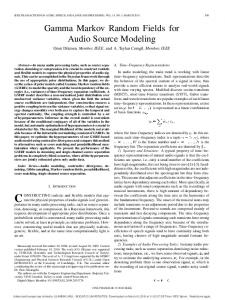
In [4], a review of an efficient algorithm solving this problem is given. 5.2. Graph Construction In our implementation, the graph G = (V, E) is constructed such that there exists a node v ∈ V for every image region at the two different region levels (high level regions and superpixels). The edges E represent the mutual dependencies between the nodes and therefore connect each two neighboring nodes at one level. By the nature of our region generation, each superpixel, belongs to exactly one high level region. In our graph, they are therefore connected to exactly this node in the higher level. Figure 2 shows a scheme of the hierarchical graphical structure used. As all five classes are present in all

5. MRF-BASED SEGMENTATION A MRF is an undirected graphical model. The graph G = (V, E)consists  of a discrete set of objects V and a set of edges |V | E ⊆ , i.e. of pairs of those objects. In our case the 2 objects or nodes v ∈ V represent the image regions. The edges represent the mutual dependencies between two nodes. In this framework, the segmentation is a labeling task where a single label xv ∈ X is assigned to each object v. The labeling is represented by a |V |-tuple x ∈ X |V | with the components xv .

Fig. 2. Hierarchical graph structure. the images, the number of labels K is constant at the superpixel level and set to five. Every node can be assigned one of the five different labels.

5.2.1. Probabilistic Data Term As stated in section 3, we can directly use the region-wise computed feature vectors to learn classifiers for the different classes. But, as there exist mutual dependencies between the different regions, we do not want to directly use the classifier to assign labels to our superpixels. Instead, we use a Support Vector Machine (SVM) to learn the local evidences (see section 4) and use these local evidences in our hierarchical MRF. When performing the classification as stated in 4, we get a probability pxv for every node v and label x.The data term gv (xv ) of the graph (G, X, g) is encoding the quality of assigning the label x to node v. We thus set gv (xv ) = pxv .

(4)

5.2.2. Edge Term In the literature (e.g. [3]), the edge term is mainly used in order to introduce smoothness into the segmentation result. In our case, this is different, because specially the small cell organelles are spread throughout the cell. A strong smoothness constraint would hamper a good classification of these organelles. Furthermore, the cell surfaces are not even and thus the cytoplasm segmentation would neither profit from a smoothness term. On the other hand, we can see that some classes are always grouped together while they never touch with others. Cell organelles for example hardly ever touch the background, while the nucleus has most common surfaces with the cytoplasm. We define the average adjacency ratio matrix AR as the symmetric matrix containing the average number of boundary pixels between class xv and class xv0 normalized by the total number of boundary pixels for all classes. The AR on the superpixel level is given in equation 5 for one example training dataset.   0.241 0.118 0 0 0.008  0.118 0.278 0.010 0.006 0.037    0.010 0.087 0 0  AR =   0  (5)  0 0.006 0 0.001 0  0.008 0.037 0 0 0.049 We base our edge term gvv0 (xv , xv0 ) on this adjacency ratio in our training data and set gvv0 (xv , xv0 ) = X xv00

2 · AR(xv , xv0 ) X (6) AR(xv00 , xv0 ) AR(xv , xv00 ) + xv00

for all v and v 0 on the superpixel level. Between the high level regions, the AR and gvv0 (xv , xv0 ) are computed accordingly. Between the two levels of hierarchy, we also have to set the edge qualities according to figure 2. Here, we base our choice on the learned distributions in the classes 10 , 20 , and 30 (see table 1). The edge between the high level node v¯ and the low

level node v is set to the corresponding class distribution entry dxv¯ ,xv , gv¯v (xv¯ , xv ) = dxv¯ ,xv . (7) 6. EXPERIMENTS Our data consists of 27 Transmission Electron Microscopic recordings from Mast Cells, more specifically BMMC (Bone Marrow-derived Mast Cells). The image size is 1024 × 1024 pixels with a resolution of 11.6 × 11.6nm2 per pixel. The data has been manually annotated by experts, who distinguished between five classes: background, cytoplasm, nucleus, mitochondria and other vesicles. This last class is the least homogeneous as it contains many different cell organelles as lysosomes the Golgi apparatus, the endoplasmic reticulum, etc. and was therefore hard to classify for the SVM. On average, the UCM yielded 1642 superpixels per image. The average number of high level regions was 43. We trained RBF-Kernel SVMs for each two class problem. The cost values were adapted with a gridsearch on one of the training images. The code of the MAX-SUM solver was downloaded from [13]. We have divided our data into three independent sets of images (each containing 9 images). The algorithm was evaluated with a three-fold cross-validation. The results were compared with those we could achieve by directly using the SVM classification (as described in section 4), as well as those we could achieve by using a simple MRF without hierarchy. For this, we built a MRF only containing the lower level of our region hierarchy. All further parameters of the MRF were chosen identically to our HMRF. 7. RESULTS As a performance measure, we use the segmentation accuracy of all classes (including background). The accuracy is computed by tp (8) accuracy = tp + fp + fn where tp, fp, and fn are the true positives, false positives and false negatives respectively. The segmentation accuracies per class are given in table 2. Additionally, we compute the overall segmentation accuracy for all classes. This might be interesting, as the classes are very different in size. Thus at visual inspection, a segmentation result with low accuracy in the cytoplasm class appears much less reasonable than a low accuracy in the mitochondria class. The overall segmentation accuracy of our HMRF segmentation is at 65.42%. With a direct SVM segmentation, one could reach 60.5%, with a simple MRF without hierarchy 61.5%. The accuracy is reasonably high for the classes background and cytoplasm (class 1 and 2). This is important because those are the largest classes and from the biological point of view, the delineation between cell and background is crucial. In the

HMRF MRF SVM

Table 2. Segmentation accuracy. accuracy in class 1 2 3 4 87.3% 61.7% 31.8% 8.1% 83.5% 58.6% 21.9% 10.8% 85.2% 57.3% 22.2% 9.5%

9. REFERENCES 5 10.9% 14.9% 17.6%

Table 3. Precision and Recall of the HMRF method. 1 2 3 4 5 precision 93.3% 67.4% 55.5% 22.7% 69.3% recall 93.3% 89.1% 40.4% 18.2% 11.9% smaller classes mitochondria and other vesicles (4 and 5), the accuracy is quite low. In order to quantify what this means, we are looking at the precision and recall precision =

tp tp + fp

recall =

tp tp + fn

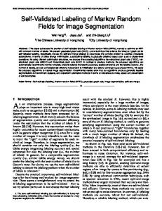
of the superpixel classification (see table 3). Here, we can see that for the vesicles (class 5) the precision is quite high while the recall is low. This means that whenever our algorithm classifies a region as vesicle, it is probably right, whereas many true vesicles are not recognized. On the other hand, the precision for the cytoplasm class is lower than its recall. This indicates that regions belonging to different classes (in our case to cell organelles), have been wrongly classified as cytoplasm. When looking at the class-wise accuracy, the SVM segmentation result seems to be already pretty good. However, when looking at the actual segmentation masks (see figure 3), one can see that the HMRF approach leads to less cluttered regions than both the other methods (SVM and MRF), which is favorable for the organelle segmentation task. Especially in the SVM classification, cell organelles as vesicles or mitochondria are detected outside the cytoplasm or on the microvilli (the tail-like extensions of the cells) which, from a biological point of view, makes no sense. With our hierarchical method this was not the case. Thanks to the global knowledge introduced by the hierarchy, specially the cell nuclei have been much better segmented, which, when looking at a small region only, is indeed really difficult.

[1] P. Arbela´ez, M. Maire, C. Fowlkes, and J. Malik, “From contours to regions: An empirical evaluation,” in Proc. of the CVPR, 2009. [2] Vladimir N. Vapnik, Statistical Learning Theory, Wiley-Interscience, 1998. [3] B. Miˇcuˇs´ık and T. Pajdla, “Multi-label image segmentation via max-sum solver,” in Proc. of the CVPR, 2007. [4] T. Werner, “A linear programming approach to maxsum problem: A review,” Trans. on PAMI, vol. 29/7, pp. 1165–1178, 2007. [5] Y Boykov and V. Kolmogorov, “An experimental comparison of min-cut/max-flow algorithms for energy minimization in vision,” Trans. on PAMI, vol. 26/9, pp. 1124–1137, 2004. [6] H. Chang, M. Auer, and B. Parvin, “Structural annotation of em images by graph cut,” in IEEE Int. Symp. on Biomedical Imaging-from nano to macro (ISBI). 2009, IEEE Computer Society. [7] C. D’Elia, G. Poggi, and G. Scarpa, “A tree-structured markov random field model for bayesian image segmentation,” Trans. on IP, vol. 12/10, pp. 1259–1273, 2003. [8] N. Plath, M. Toussaint, and S. Nakajima, “Multi-class image segmentation using conditional random fields and global classification,” in Proceedings of the 26th Annual International Conference on Machine Learning, New York, NY, USA, 2009, ICML ’09, pp. 817–824, ACM. [9] J. Reynolds and K. Murphy, “Figure-ground segmentation using a hierarchical conditional random field,” in Proceedings of the Fourth Canadian Conference on Computer and Robot Vision, 2007. [10] J. Shotton, M. Johnson, and R. Cipolla, “Semantic texton forests for image categorization and segmentation,” in Proc. of the CVPR, 2008. [11] M. Maire, P. Arbela´ez, C. Fowlkes, and J. Malik, “Using contours to detect and localize junctions in natural images,” in Proc. of the CVPR, 2008.

8. CONCLUSION We have presented a multi-label segmentation algorithm based on a hierarchical graphical model. We could show that our method outperforms the local region classification by SVMs as well as classical MRF regarding the overall classification accuracy. Compared to classical MRFs, the region consistency reached with our method is much higher thanks to the topological knowledge introduced by the region hierarchy.

[12] T.-F. Wu, C.-J. Lin, and R. C. Weng, “Probability estimates for multi-class classification by pairwise coupling.,” Journal of Machine Learning Research, vol. 5, pp. 975–1005, 2004. [13] http://cmp.felk.cvut.cz/cmp/software/maxsum/.

Raw Data

Ground Truth

SVM

MRF

HMRF

Fig. 3. Results of the three different methods on our data. Black corresponds to the label background, yellow to cytoplasm, red to nucleus, cyan to mitochondria and blue to vesicles. The results of our method, displayed in the last column, are the most consistent.