IEMS Vol. 7, No. 2, pp. 160-170, September 2008.
A Mathematical Model for Converting Conveyor Assembly Line to Cellular Manufacturing Ikou Kaku† Department of Management Science and Engineering, Akita Prefectural University, Yulihonjo, 015-0055, JAPAN Tel: +81-184-27-2171, Fax: +81-184-27-2189, E-mail:
[email protected] Jun Gong Institute of Systems Engineering, Key Laboratory of Integrated Automation of Process Industry of MOE, Northeastern University, Shenyang 110004, P.R.CHINA Tel: +86-24-23264336, +86-24-83680568, E-mail:
[email protected] Jiafu Tang Institute of Systems Engineering, Key Laboratory of Integrated Automation of Process Industry of MOE, Northeastern University, Shenyang 110004, P.R.CHINA Tel: +86-24-23264336, +86-24-83680568, E-mail:
[email protected] Yong Yin Department of Economics and Business Management, Yamagata University, Yamagata, 990-8560 JAPAN Tel: +81-23-628-4281, E-mail:
[email protected] Selected paper from APIEM 2006 Abstract. This paper proposes a mathematical model for converting conveyor assembly line to cellular manufacturing in complex production environments. Complex production environments refer to the situations with multi-products, variant demand, different batch sizes and the worker abilities varying with work stations and products respectively. The model proposed in this paper aims to determine (1) how many cells should be formatted; (2) how many workers should be assigned in each cell; (3) and how many workers should be rested in shortened conveyor line when a conveyor assembly line should be converted, in order to optimize system performances which are defined as the total throughput time and total labor power. We refer the model to a new production system. Such model can be used as an evaluation tool in the cases of (i) when a company wants to change its production system (usually a belt conveyor line) to a new one (including cell manufacturing); (ii) when a company wants to evaluate the performance of its converted system. Simulation experiments based on the data collected from the previous documents are used to estimate the marginal impact that each factor change has had on the estimated performance improvement resulting from the conversion. Keywords: Line-cell Conversion, Cellular Manufacturing, Conveyer Assembly Line, Mathematical model
1. INTRODUCTION Cellular manufacturing (CM) is a manufacturing system in which one (or multiple) worker carries out all of the operations of a job, usually in a U-shaped layout. Since it seems to be able to improve system perform† : Corresponding Author
ance in a changing environment, many Japanese companies have introduced CM into their factories to convert existent conveyor assembly line (CAL). An early document about such line-cell conversion was reported by Tsuru (1998), which is based on a questionnaire of 13 factories and one consulting company. These anonymous
A Mathematical Model for Converting Conveyor Assembly Line to Cellular Manufacturing
factories converged in electronic and automobile industries. The main standpoint of the document claimed that CM can be recognized as a form of the knowledge of Toyota Production System which has been historically transferred to other industries. In recent years, after many Japanese companies shifted their production organizations to China, those manufacturers left behind in Japan have been changing their production ways remarkably. Several manufacturing methods have been developed for strengthening their competitive power of the domestic companies. In addition, instead conveyor mass production, only the products what suited the needs of customers (the kinds of products are changing dynamically) should be manufactured flexibly when they were needed (the production quantities are also variables). For example, Tanaka (2005) reported that there are seven manufacturing methods have been used to correspond so-called new manufacturing in RICOH UNITECHNO Inc., which is a middle scale Japanese company to manufacture facsimiles/copy machines/printers. Those methods are as follows: (1) One worker-One machine method (the product will be assembled by only one worker, he should do all of the assembly operations); (2) Two workers-One machine method (there are too operational works to assemble for a larger machine that can not complete by one worker, in such case two workers should be assigned to do this assembly operation); (3) Cart pulling method (instead conveyor line a cart is used as transport tool, which is pulled among several workers to complete the assembly operations); (4) Relay method (the form of assembly line is existed but the workers assigned in the line do not only those operations for themselves but also the operations not assigned for them, by their operation ability); (5) Conveyor assembly line (traditional assembly method is also remained for those large lot size products); (6) One worker CM (only one worker does all of the assembly operations of products usually in a U-shaped layout. The difference with method (1) is that the worker in the CM can do all of assembly operations of several products, that means he has a higher operation ability.); (7) Division CM (several workers are assigned in one cell, they may do the assembly operations using the methods of (3), (4) or (6)). Those methods and their combinations are used to correspond flexibly different kinds (over 400 kinds of products) and different quantities (70% of products are under 100 units/month) of products, and successful performances were gained. It should be pointed that all of these innovations in Japan industries are based on the reflection of mass conveyor manufacturing and are for searching more effective production systems. Converting old conveyor assembly line to new manufacturing systems are not the goal but only the ways and means to increase the productivity of companies. A tremendous achievement of such conversion is brought from CANON Inc., a famous Japanese electronic company. Takahashi, Tamiya and Tahoku (2003) reported that by introducing CM into their factories in CANON,
161
since 1995 there are over 20,000 meters of belt conveyor have been withdrawn and 720,000 square meters of working space from 54 related factories were emptied. The total cost rate was decreased from 62% to 50% during past eight years. Since then converting CAL in Japanese manufacturers is coming into fashion. Yin, Kaku and Murase (2006) pointed out the economic background of converting CAL to CM in Japan based on a survey of last Japanese literature. Summarily, Japanese manufacturers were faced with a decreased market demands and increased product variations. To survive in such an extremely tough business environment, the traditional high-volume conveyor assembly lines were no longer fulfilled. Speedy adjustments were needed to handle transitions in product models and demands. A company’s competitiveness was becoming dependent on whether or not it can respond to these transitions. In such an environment, there was a trend in Japanese industries toward converting conveyor assembly lines to more flexible manufacturing cells. Basically, the term of CM is not a new concept. Over the previous decade, a series of research articles have investigated CM systems and compared the performance of traditional function layout and CM systems. For example, Wemmerlöv and Hyer (1989), Wemmerlöv and Johnson (1997), Johnson (2005) claimed that CM represents a major technological innovation to many manufacturing systems traditionally based on functional or assembly specialization. As a result, many manufacturing organizations with traditional function layout manufacturing systems have either already adopted CM or are considering their adoption. Sakazume (2005) investigated a survey of Japanese literature that included total 107 documents (12 academics, 18 technical reports and 77 newspaper articles). Through comparing their advantages and disadvantages, he tried to explain that the so-called American Cellular Manufacturing (from traditional function layout to cells) and Japanese Cell Manufacturing (from belt conveyor line to cells) are completely different in term of implementation changes and mechanisms, even through there are some similarities in term of cell features and implementation. Johnson (2005) used a previous theory to explain why the assembly cells are expected to outperform the current assembly line. He investigated simulation models to estimate the marginal impact that the operational factor change had on the estimated performance improvement resulting from the conversion. Kaku, Murase and Yin (2008) proposed a theoretical model of the conversion involved human factors. Because the performance improvement resulting from the conversion is dependent on those operating factors that can improve the system performance and overcome any task time increases caused by the loss of worker specialization, the cross-training of workers should be considered to be a key issue in the conversion. They investigated a theoretical model to analyze the cross-training of workers quantitatively by using human memory ability and to suggest that infor-
162
Ikou Kaku ᆞ Jun Gong ᆞ Jiafu Tang ᆞ Yong Yin
mation support system can improve the cross-training effect. However, it should be attended that converting CAL to CM is a new concept. When an assembly line is converted to cells, each cell performs the tasks formerly assigned to numerous stations on the line. Depending on the job design, each worker assembles either a portion or all of the subassembly or product produced in the cell, may also be responsible for dynamically balancing the flow of work as product mix or demand levels change. On the other hand, the increased number of assembly tasks performed by each cell worker may increase the time required for each task, which serves to hinder the performance improvement caused by cell conversion. Moreover, because all of workers in assembly line were not able to have same skill performing those assembly works, some workers are not appropriate doing those tasks assigned in cells. Those cause resulted some companies did not lead to performance improvements with converting their assembly lines to cells. Therefore, how to convert their CAL to CM is a very complicate decision problem for those companies who wanted to do such conversion. There are several researches reported the advantages and disadvantages of converting CAL to CM (see Tsuru 1998, Isa and Tsuru 1999, Sakazume 2005, Miyake 2006) but those proposed suggestions are not appropriate to support such decision. Our objective is to build up a mathematical model to describe the line-cell conversion problem and to analyze the system performance of such conversion in a complex production environment. In this paper, the complex production environment is considered as a situation with multi-products, variant demand, different batch sizes and variable worker abilities with work stations and products respectively. The remainder of this paper is organized in the following way. We give a brief description of the conversion problem and then build the mathematical model in next section. The simulation experiments are designed in the third section. The result analysis and discussions are given in the fourth section. Concluding remarks are given in the final section.
2. PROBLEM DESCRIPTION AND MATHEMATICAL MODEL We consider following production problem: there exist a traditional belt conveyor line with multiple assembly stations. Workers were assigned at each station according to a traditional job design method but they have had ability to do more tasks than that were assigned to them. We assume that the worker’s abilities are different with stations and products. Multiple products will be manufactured in the conveyor line, each product is able to have different batch sizes but with a known distribution of demand. Products should be manufactured by a given scheduling rule like as First Come
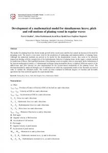
First Service (FCFS) but with a full batch (i.e., the batch splitting is not permitted). When the products are assembled in the conveyor line, the stations and workers used to complete the assembly jobs are active. Because workers have different abilities to do those jobs (which belong to stations and products) when the batch will be finished is dependent on the worker with slowest speed to do the jobs. That means the abilities of the other workers were not useful sufficiently, which may lead to decreasing the motivation of workers. On the other hand, all of the products should be manufactured at the same conveyor line with a fixed order; there may be some waiting times in the manufacturing so that we can not response flexibly to the customer’s variant demand. In this paper, we propose KAIZEN methods to improve the system performance of such conveyor line. Assume that the workers will do all of jobs that they can do even that are not assigned for them, there are several KAIZEN methods to implement the conveyor line. For example, workers who have higher abilities should help other workers in the conveyor line; or converting the conveyor line to some assembly cells; or converting part of line to cells for workers who have higher abilities and remain the part of conveyor line for workers who have lower abilities. In this paper, we consider three types of production systems including pure CM, pure CAL and a hybrid type of CM+CAL. It does not influence the system performance either CM is set to front or behind of CAL (Van der Zee and Gaalman 2006). For simplicity and without lose of generality, we assume CAL is formatted behind CM in the hybrid production system as shown in Figure 1. We propose a two step approach to design the production system from Figure 1. First step is a cell formation approach: if there were only cells formatted in the system (pure CM), we assign all of workers to cells according to their abilities which are different with products and stations; if there were part of CAL be converted to cells, we assign the workers with higher abilities to cells and remain the workers with lower abilities to CAL. The case of workers can help each other in the conveyor line just should be considered like as a pure CM in which all workers in CAL are assigned in cells. Finally, the pure CAL is the traditional belt conveyor line. The second step is a scheduling approach: a first come first service (FCFS) rule is used to assign product batches to cells or CAL. In the case of pure CAL the product batches are just scheduled according to the order of their coming; in the case of pure CM the product batches are scheduled according to not only the order of their coming but also the ability of workers (that means that product should be assigned prior to the worker (cell) who has higher ability to do the job). In the case of hybrid system of CAL+CM, the product batches are firstly assigned to cells with the FCFS rule, then assigned to CAL with the order calculated by the earliest finish time rule.
163
A Mathematical Model for Converting Conveyor Assembly Line to Cellular Manufacturing
1
2
…
3
W
Cell 1
1
M 2
Cell 2
·· ·
·· ·
M
Cell J
…
2
1
CAL
Worker
Product batch
Worker assign
Batch assign
Figure 1. A hybrid production system of CM + CAL. No. of Cell
3
3
4
3 2
1
2
4
2
2 1
No. of Cell
4
1
3 1 Time
Time CAL
CELL m
Product batch m
Figure 2. A case of scheduling in the hybrid production system Figure 2 shows an example of the case of CAL + CM with four batches and three cells, where the length of rectangle chart in Figure 2 states the flow time of a product batch. For evaluating the system performance two criteria are considered. Firstly we define total throughput time to represent the system productivity that is the time of all of product batches had been finished. That is to say, for given product mix the new production system should have a shorter total throughput time. Secondly we define total labor power (hours) to represent the work efficiency that is the cumulative working time of all of workers assigned in the system. Therefore, our problem is to determine the number of cells and number of workers in each cell to minimize the total throughput time and total labor power. 2.1 Problem features and assumption Following assumptions are considered in this paper to construct the model: 1) Multiple products are planed to assembly with a pro-uct mix.
2) Products are assembled with different batches and diferent batch sizes. 3) Types and batches of products are known and constant. 4) Number of tasks is the same to all of product types. (If the number of tasks were different with products then assume the task time to do the different tasks was zero so that we can treat the products with different assembly tasks). 5) If the production system is CAL, just one CAL is considered. 6) Number of workers is the same with the number of tasks on CAL. 7) A worker only does a task in CAL. 8) Number of workers in each cell may be different but limited. 9) Number of tasks assigned to each cell is the same. 10) Number of tasks assigned to each cell is at least greater than a constant. 11) A worker assigned in a cell can operate all the tasks assigned in the cell. 12) A product batch is just processed in a cell. 13) Setup time is considered when two different types of
164
Ikou Kaku ᆞ Jun Gong ᆞ Jiafu Tang ᆞ Yong Yin
products have been assigned into a cell, but the setup time between two batches with the same product type is zero. 2.2 Notations We define the following terms: • Indices i : Index set of workers (i = 1, 2, " , W ) . j : Index set of cells ( j = 1, 2, " , W ) . n : Index set of product types (n = 1, 2, " , W ) . m : Index set of product batches (m = 1, 2, " , W ) .
the system which may be pure CM or pure CAL or a hybrid type of CM+CAL system. Given the upper bound Wmax on the number of workers and the lower bound S min on the number of stations (tasks) in one cell, the objective is to determine the number of cells and workers in each cell to minimize the total throughput time and the total labor hours. The comprehensive mathematical model is given in Equations (1)-(7) as below.
{
• Decision variables X ij = 1, if worker i is assigned to cell j , otherwise 0. Yi =1, if worker i is assigned to CAL, otherwise 0. Pmj =1, if product batch m is assigned to cell j , otherwise 0. Lmr =1, if product batch m is assembled by order r on CAL, otherwise 0. Z= 1, if CAL exists in the system, otherwise 0. • Variables Ci : Coefficient of variation of assembly task time of worker i in each cell accounting for the effect of multiple stations. CTm : Actual cycle time of product batch m in CM. FCm : Flow time of product batch m in CM. FCBm : Begins time of product batch m in CM. LTm : Actual cycle time of product batch m on CAL. FLm : Flow time of product batch m on CAL. FLBm : Begin time of product batch m on CAL. 2.3 Problem formulation Here we consider the production planning problem which is based on a fixed product mix with M product batches and N product types. W workers are assigned to
m
M
W
J
Z 2 = Min ∑ ∑ ( ∑ Pmj FC m X ij + FLm Yi ) m = 1 i =1
J
• Parameters Wmax : Maximum number of workers in one cell. Smin : Minimum number of stations in one cell. TBnm : A 0-1 binary variable where TBnm = 1 , if product batch m is for product type n ; otherwise 0. Bm : Size of product batch m . Tn : Standard assembly time to each task of product type n at each station. LSn : Setup time of product type n on CAL. CS n : Setup time of product type n in CM. ε i : Coefficient of influencing level of skill to multiple stations for worker i . ηi : Upper bound on the number of tasks for worker i in one cell, if the number of tasks assigned to workers is over than it, the task time will become longer than ever. β ni : Level of skill to for worker i for one task for product type n .
}
Z1 = Min Max [ (1 − Z )( FCBm + FCm ) + Z ( FLBm + FLm )] (1)
∑
X
j =1 W
∑Y i =1
W
∑
i
ij
W
∑
i =1
X
+ Yi ≤ 1
∀i
ij
⎧ ⎪1 ⎪ Z =⎨ ⎪0 ⎪⎩
≤ W m ax ≤
W
∑
X
i =1
il
W
∑Y i =1 W
(3) (4)
≤ W − S m in
X
i =1
ij
(2)
j =1
i
∀j ∀ j > l , ( l = 1, 2 , " , J )
(5) (6)
≥1
∑ Yi = 0
(7)
i =1
Where, equation (1) states the objective to minimize the total throughput time of the total product batches assignments. The total throughput time is the due time of the last completed product batch. The first part is the throughput time in CM. The second part is the throughput time in CAL. Equation (2) states the objective to minimize the total labor power (hours) of the product batches assignments. The total labor power is the time of all of workers manufactured all of the product batches. The first part is the labor hours in CM. The second part is the labor hours on CAL. Because the objective functions are too long to write, the detail definition of the objective functions are represented in the following subsections. Equation (3) is the rule of worker assignment ensures that each worker should be at most assigned to one cell or CAL. The sign of inequality means that the worker who has the worse ability is discarded possibly. Equation (4) is a minimum number of tasks in each cell which means if there is no task in cells, the production system will become traditional CAL. Equation (5) is a cell size constraint because the space of a cell is limited. The value of the maximum number of workers in one cell will be a function of plant size, design and process technology. Equation (6) is the rule of cell formation ensures that the number of workers in prior cell is greater than that in next cell. Equation (7) is a flag variable shown whether the CAL exists in the system. This rule can lead a smaller search space of feasible solutions but guarantee the optimality of solutions.
A Mathematical Model for Converting Conveyor Assembly Line to Cellular Manufacturing
2.3.1 Scheduling of batch production in CM For defining the objective function in CM, the production plan will be scheduled with a given scheduling rule under the worker assignments to CM. Firstly, a worker’s level of skill is able to vary with the number of tasks. If the number of tasks is over an upper bound ηi , the task time will become longer. This can be represented as below:
C i = 1 + ε i m a x ( (W −
W
∑Y i =1
i
− η i ), 0 )
(8)
Secondly, the assemble task times of a product is also able to vary with workers. Consequently, the task time of a product is calculated by mean task time of all workers in the same cell. Actually, the task time of product batch m is represented via following equation: W
C Tm =
J
N
∑ ∑ ∑ i =1
j =1 n =1 W
T n β n i T B m n Pm j C i X J
∑ ∑ i =1
j =1
Pm j X
ij
(9)
J
∑
j =1
m
M
∑∑ s =1
j =1
Pm j = 1
∑C m =1
mj
=0
W
∑X i =1
ij
∀m
(10)
N
∑
n =1
m a x (T n β n i T B m n Y i )
N ⎧W N ⎪∑Yi ∑Tn βniTBmn + LTm (BSm −1) + ∑ LSn (1− TB(m−1)nTBmn ) m > 1 ⎪ i =1 n=1 n=1 FLm = ⎨ W N N ⎪ Y T β TB + LT (BS −1) + LS TB m =1 ∑ i ∑ n ni mn m m n mn ⎪⎩∑ i =1 n =1 n=1
FLBm = max(FCBm + FCm , FLBK + FLK ) M
(11) (12)
∀m
(13)
= 0, ∀ j
(14)
Where, equation (10) states the flow time of product batch m . The first part is the process time and the ⎡ ⎤ ⎢ ⎥ B ⎥ second part is the setup time, where ⎢ W J m ⎢ ⎥ ⎢ ∑∑ Pmj X ij ⎥ ⎢ i =1 j =1 ⎥ presents the upper integer number of products for each worker in the same cell. Equation (11) states the begin time of each product batch. There is no wait time between two product batches so that the begin time of one product batch is aggregation of flow time of all of the
(15)
Then, using the FCFS rule, the flow time FLm and begin time FLBm of product batch m is presented as below.
∑
m =1
M
∀m
FCBm ≤ FCBm +1 M
F C m P s j Pm j
2.3.2 Scheduling of batches production in CAL For defining the total throughput time of the product batch assignments in CAL, the production plan will be scheduled with a given scheduling rule under the worker assignments to CAL. Of course, if all workers are assigned to CAL, that is the traditional production system, otherwise, that is CM+CAL hybrid production system. Here, the task time is calculated by the longest task time among the workers on CAL. Actually, the task time of product batch m is represented via the following equation: L Tm =
⎧ ⎡ ⎤ ⎪ ⎢ ⎥ N W J Bm ⎪CT (W − ∑ Y ) ⎢ ⎥ + ∑ CS n (1 − ∑ TB( m −1)TBmn P( m −1) Pmj ) m > 1 m i W J ⎪ ⎢ ⎥ n i =1 j =1 P X ∑ ∑ mj ij ⎥ ⎪ ⎢ ⎪ ⎢ i =1 j =1 ⎥ FCm = ⎨ ⎡ ⎤ ⎪ ⎢ ⎥ N W J ⎪ B ⎥ + ∑ CS n ∑ TBmn Pmj m =1 ⎪CTm (W − ∑ Yi ) ⎢ W J m ⎢ ⎥ n i =1 j =1 ⎪ P X ⎢ ∑ ∑ mj ij ⎥ ⎪ ⎢ i =1 j =1 ⎥ ⎩
FC Bm =
prior product batches which are in the same cell. Equation (12) is the assignment rule in which a product batch is just only assigned to a cell. Equation (13) is the FCFS scheduling rule which means the prior product batch must be assembled before the next product batch. Equation (14) are the rules of assigning constraints, that means a product must be assigned to a cell in which a worker is assigned at least.
ij
Then, using the FCFS rule, the flow time FCm and begin time FCBm of product batch m is represented as below.
165
∑
r =1
⎧⎪ Lmr = 1, LK (r −1) = 1 r > 1 ⎨K r =1 ⎪⎩ Lkr = 1
(16)
(17)
Lmr = 1
(18)
Lmr = 1
(19)
Lm1r FLBm1 ≥ Lm2 (r −1) (FLBm2 + TLm2 )
∀m1 , m2 ∈ M
(20)
Where, equation (16) states the flow time of product batch m , the prior two parts are the flow time of product batch m , the third part is the setup time of product batch m . Equation (17) states the begin time of each product batch. If the production system is the hybrid CM+CAL model, the waiting time between two product batches will be considered, otherwise no consideration for waiting time. In the hybrid CM+CAL model, the begin time of product batch m is the maximum value between the end time of the prior product batch on CAL and the end time of product batch m in CM. In the CAL model, the begin time of product m is the end time of the prior product batch which is ordered by the FCFS rule. Equation (18) ensures that a product batch is must assigned to an order. Equation (19) ensures that a order is must assigned with a product
166
Ikou Kaku ᆞ Jun Gong ᆞ Jiafu Tang ᆞ Yong Yin
batch. Equation (20) ensures that the begin time of a product batch must be late the end time of the prior product batch.
3. NUMERICAL SIMULATIONS By using formula (1)-(20), the line-cell conversion problem can be described completely that whether the conveyer assembly line should be converted to cell(s) and how to do such conversion. In the hybrid model, for a given number of workers (X + Y), the objective functions are not linear but bounded. Hence, we must conduct an exhaustive search over X + Y. Since there are (X + Y) major loops for cell formation and J minor loops for scheduling, for practical values of X + Y and J it is not computationally intensive. The purpose of this paper is to compare the performances of CM and CAL under complex production environments. Therefore we do numerical experiments to simulate the effects of each of factors influenced on the performance of production system based on the mathematical model proposed above. For comparison of the performance between new production system and CAL, the percentage changes are defined as below. For simple representation, we shorten the total throughput time as TTPH and the total labor power (hours) as TLH as following. TTPH = (
TLH = (
TTPH of C M − TTPH of C AL ) *100 TTPH of C AL
TLH of C M − TLH of C AL ) *100 TLH of C AL
Clearly, the percentage changes of TTPH and TLH of pure assembly line are zero. 3.1 Parameter design
Tables 1 and 2 show the parameters used in the experiments. As shown in Table 1, the parameters in first and second row are factors influencing the level of skill to multiple tasks for worker i . ηi is the upper bound on the number of tasks for worker i in a cell, which is assumed to be 10. If the number of tasks assigned to a worker is over than it, the task time will become longer than ever. ε i is used to control the variability of level of worker’s skill, which is based on a normal distribution with a mean value 0.2 and a standard deviation 0.05. Simply, the inter-arrival time is neglected here. The parameters in third and fourth row are the setup times in CM and CAL which shows that the setup time in CM is smaller than that in CAL. The values of them are separately 1 minute and 2.2 minutes. The setup time in the joint model CM+CAL is considered as the same with CAL. The parameter in fifth row is the standard task time, which is assumed to be 1.8 minutes. The parame-
ters in sixth and seventh row are the maximum number of workers in a cell and minimum number of tasks needed in a cell. The values of 5 and 2 are assumed. Finally, the parameter in eighth row is the number of cells which is given by 10, because the biggest number of tasks in this experiment is 20 and 2 tasks must be assigned to each cell at least, the value over 10 is meaningless. As shown in Table 2, the worker’s level of skill can be considered to be able to vary with product types. In our simulation experiments the variation is assumed to be a normal distribution with the mean value 1 and the range of standard deviation from 0.1 to 0.3. The more the product types will be manufactured, the larger the variation of worker’s skill. 3.2 Factors design
For comparing the performances among the different production system, four kinds of hybrid system were considered, which included Best CM (optimal solution), 2 workers CM (two workers were forced to be in a cell), 3 workers CM (three workers were forced to be in a cell) and 6 workers CM (six workers were forced to be in a cell). There are a lot of our side and inside factors which can influence the system performance. A brief overview of four factors used in the experiments is given in Table 3. 3.2.1 Product type Since CAL is designed for single product at first, it can be considered that the performances of CAL will become worse when the product type changes to be multiple. We set five cases, in which the number of product type ranged from 1 to 5, to confirm this supposition. In this way, the higher variability of worker’s level of skill will happen with more product types in the production system according to the parameters set above. 3.2.2 Product batch Even CAL is considered be suitable to single (less) product type, product batch is still influencing the system performances. It can be considered that CAL is better in a less product batch environment, and become worse when the product batches increase. From this view point, five cases of different number of product batches are arranged for investigating the effects of product batches, which are assumed be from 3 to 7. 3.2.3 Batch size Batch size can be considered as a factor that influences the system performances mostly. The performances of CAL will become worse when the batch size of the product changes to be smaller. We set five cases in which the batch size were set to be from 10 to 200. In this way, the effects on the system performances with different volume of batch sizes can be investigated.
167
A Mathematical Model for Converting Conveyor Assembly Line to Cellular Manufacturing
3.2.4 Task size Distinguish the outside factors above, cross-training of workers is a significant inside factor which can influence the system performances of hybrid systems. Through cross-training methodology, the worker’s level of skill to deal with multiple tasks should become higher and higher.
4.1 Product type
Figure 3 and 4 showed the percentage changes of the two system performances measures with the increasing of product types. Figure 3 shows the percentage changes of total throughput time (TTPH) and Figure 4 shows the percentage changes of the total labor hours (TLH).
Table1. Experimental parameters. Parameter
Value
ηi
10
εi
N(0.2, 0.05)
CAL( LS n )
2.2 minutes
CM ( CS n )
1 minute
( Tn )
1.8 minutes
Wmax
5
S min
2
J
10
Note) N(0.2, 0.05): Normal distribution( μ = 0.2, σ = 0.05 ).
Table 2. Worker’s level of skill ( β ni ) with product types.
Figure 3. TTPH with different product types.
Product Type 1
2
N(1, 0.1)
N(1, 0.15)
N(1, 0.2)
N(1, 0.25)
N(1, 0.3)
Note) N(1, 0.1): Normal distribution( μ = 1, σ = 0.1 ).
According to this consideration, the different values of task size are assumed from 4 to 20, while the lower bound on the number of multiple tasks is fixed to be 10. If the task size is greater than 10, the standard task time will become longer. The effect of worker’s ability to deal with multiple tasks on the performances of the hybrid systems will be investigated in the experiments.
4. RESULTS AND ANALYSIS Several simulation results are obtained from our experiments. Here we show some main observations from the standpoint of minimization of total throughput time with the constraint of the total labor hours.
Figure 4. TLH with different product types.
From the viewpoint of TTPH Figure 3, generally the percentage changes of all the CM systems are decreasing when the product types are increasing. That means increasing of product types leads to better performance in CM but worse performance in CAL. However, except Best CM, the performances of 2 workers CM, 3 workers CM, 6 workers CM are not able to ex-
Table 3. Experimental factors Factor
Product Type
Product Batch
Product Type Product Batch Batch Size Task Size
1, 1-2, 1-3, 1-4, 1-5 1 1 1
6 3, 4, 5, 6, 7 6 5
Batch Size
Task Size
50 12 N(50,5) 12 N(10, 5), N(30, 5), N(50, 5), N(100, 5), N(200, 5) 12 N(50, 5) 5, 10, 12, 15, 20
168
Ikou Kaku ᆞ Jun Gong ᆞ Jiafu Tang ᆞ Yong Yin
ceed that of CAL in the experimental situations. The solution of Best CM is varying with product types, especially when the product type is 5 the Best CM is constructed with two 5 workers CM + 2 workers CAL and achieve maximum 15% improvement in total throughput time. It should be noticed that all of the workers in CAL also be assigned in the Best CM. But in the case of Best CM, several workers do their jobs each other according to their abilities and only the workers who have not had cross training were remained at rested CAL. Considering the constraint of TLH Figure 4, increasing of product types also leads to better performance in CM than that in CAL. When product types are over 4, all of CM systems can improve the performance of total labor hours in the experimental situations. 4.2 Product batch
Figure 5 and 6 showed the percentage changes of the two system performances measures with the same product type and the increasing of product batch. Figure 5 shows the percentage changes of total throughput time (TTPH) and Figure 6 shows the percentage changes of the total labor hours (TLH).
Figure 5. TTPH with different product batches.
From the viewpoint of TTPH Figure 5, because CAL is originally designed for single product type rather than CM, the performances of CM systems are varying significantly but can not exceed that of CAL. Especially it can be observed from Figure 5 when the product batch is more than 5 the Best CM can achieve performance improvement in total throughput time. The solution of Best CM is constructed with two cells in which 9 workers were assigned and 2 workers were remained in CAL. Considering the constraint of TLH Figure 6, increasing product batch is not able to lead to better performance in almost of CM systems except the Best CM. When product batch is more than 4 the Best CM can achieve about 25% performance improvement in total labor hours in the experimental situations.
4.3 Batch size
Figure 7 and 8 showed the percentage changes of the two system performances measures with the increasing of batch size. Figure 7 shows the percentage changes of total throughput time (TTPH) and Figure 8 shows the percentage changes of the total labor hours (TLH). From the viewpoint of TTPH Figure 7, when the batch size is small (