Vol. 57, 2011, No. 3: 110–115
Res. Agr. Eng.
A mathematical model for predicting the cracking efficiency of vertical-shaft centrifugal palm nut cracker M.C. Ndukwu1, S.N. Asoegwu2 1
Department of Agricultural Engineering, Michael Okpara University of Agriculture, Umuahia, Nigeria 2 Department of Agricultural Engineering, Federal University of Technology, Owerri, Nigeria Abstract Ndukwu M.C., Asoegwu S.N., 2011. A mathematical model for predicting the cracking efficiency of verticalshaft centrifugal palm nut cracker. Res. Agr. Eng., 57: 110–115. A mathematical model for predicting the cracking efficiency of vertical-shaft palm nut cracker was presented using dimensional analysis based on the Buckingham’s π theorem. A high coefficient of determination of 94.3% between the predicted and measured values showed that the method is good. The model was validated with data from existing palm nut cracker and there was no significant difference between the experimental cracking efficiency with the predicted values at 5% level of significance. Keywords: cracking efficiency; prediction equation; feed rate; throughput capacity; shaft speed; dimensional analysis
The modern crackers are of two types; the hammer impact and the centrifugal impact types. The hammer impact type breaks or cracks the nut on impact when the hammer falls on it; while centrifugal impact nut cracker uses centrifugal action to crack the nut (Ndukwu, Asoegwu 2010). In the centrifugal impact type; the nut is fed into the hopper and it falls into the housing where a plate attached to the rotor is rotating; which flings the nut on the cracking ring; thereby breaking the nut. Cracking therefore is an energy-involving process. According to some researchers (Asoegwu 1995; Ndukwu 1998) shelling or cracking has always posed a major problem in the processing of bio material and they attributed this to the shape and the brittleness of the kernel of the nut; rendering them susceptible to damageduring cracking. Presently most of the research work is tailored into modelling of the variables which determine the functionality of processing machines. Most of these models are specific and related to a particular design 110
of a machine. Some researchers (Degrimencioglu, Srivastava 1996; Shefii et al. 1996; Mohammed 2002; Ndirika 2006) used the dimensional analysis based on the Buckingham’s π theorem as veritable instrument in establishing a prediction equation of various systems. Therefore the present study is undertaken to establish a mathematical model for predicting the cracking efficiency of vertical-shaft centrifugal palm nut cracker using the dimensional analysis. Material and Methods Prototype of palm kernel cracker machine A centrifugal palm nut cracker prototype testing machine described in Ndukwu and Asoegwu (2010) was used in validating the model. The palm kernel cracker is powered by 1,600 kW electric motor and operates with centrifugal action. It consists
Res. Agr. Eng.
Vol. 57, 2011, No. 3: 110–115
Table 1. Dimensions of variables influencing cracking efficiency Variables
Symbol
Dimensions
Cracking efficiency (%)
CE
M 0L 0T 0
Nut moisture content (%)
Ø
M 0L 0T 0
Bulk density of the nut (kg/m3)
δ1
M1L-3T0
Nut particle density (kg/m3)
δ2
M1L-3T0
Feed rate (kg/s)
γr
M 1L 0T 1
Throughput capacity (kg/s)
Tc
M 1L 0T 1
Cracking speed (m/s)
v
M 0L 1T 1
Diameter of the cracking chamber (m)
D
M 0L 1T 0
of a conical shaped hopper that opens up into a cylindrical cracking chamber with a force-fitted mild steel cracking ring. A vertical-shaft is fitted into the cracking chamber from the bottom and is attached to a channel for directing the palm nut falling on it. The centrifugal action of the shaft flings the nut on the cracking ring with the nut cracking on impact. The palm kernel used in the experimental analysis is described in (Ndukwu, Asoegwu 2010) and is made up of a mixture of dura and ternara species of palm kernel. The diameters and thickness were determined with a vernier calliper reading up to 0.01 mm while the moisture content was determined in an oven. Model development: palm kernel cracking and separation Cracking involves all action from the hopper orifice through the cracking chamber to the collector chute. The physical quantity affecting the cracking process includes both crop physical properties and machine parameters (Ndukwu 1998; Simonyan et al. 2006; Asoegwu et al. 2010). 1. Crop properties include: crop species; age; nut moisture content; bulk density; nut geometric mean diameter.
2. The machine properties: feed rate; diameter of the cracking chamber; shaft speed; and throughput capacity. The following assumptions were made in developing the model: 1. the moisture content of the shell and kernel is the same, 2. the nut dimension is constant at the same moisture content, 3. the thickness of the shell is the same at the same moisture constant, 4. diameter of the cracking ring is fixed, 5. distance between the channel and cracking ring is fixed, 6. the age of the nut is the same, 7. the individual weight and volume of the nut is constant at a particular moisture content, 8. cracking speed is the same as the shaft speed, 9. the shaft speed is fixed. Based on the above assumptions the major variables of importance are: the nut moisture content; bulk density of the nut; nut particle density; feed rate; throughput capacity and cracking speed (Ndukwu 1998). The cracking efficiency which is the fraction of cracked and undamaged kernel recovered from the collector chute can be expressed as follows: = f �∅; δ1 ; δ2 ; γr ; v; D; Tc�
(1)
where: CE – cracking efficiency (%) Ø – nut moisture content (%) δ1 – bulk density of the nut (kg/m3) δ2 – nut particle density (kg/m3) γr – feed rate (kg/s) Tc – throughput capacity (kg/s) v – cracking speed (m/s) D – diameter of the cracking chamber (m)
The dimensions of the variables is presented in Table 1. The number of variables of importance that determines the cracking efficiency (CE) is 7 and the
Table 2. The dimensional matrix of variables is given as follows Ø
δ1
δ2
γr
Tc
v
D
M
0
1
1
1
1
0
0
L
0
–3
–3
0
0
1
1
T
0
0
0
1
1
1
0
111
Efficiency (%)
Efficiency (%)
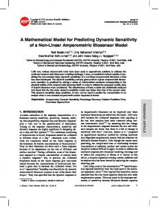
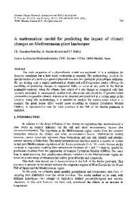
; ;Tδ; ;δ 𝑇𝑣; ;𝑇 𝐷) ;𝐷) =𝐷) 0==0=0 0 �� �𝑇 ;γ�;rγ;;γrγr𝑣; ; ;r𝑣; 𝑓(δ ;𝑣; = f �δ1 ; δ2 ; γ𝑓(δ ;𝑓(δ v; ;;�δ�D� � �;𝑇;�𝐷) c�δ �� r𝑓(δ D = L (1) = f δ ; δ ; γ ; v; D; T= �∅; ; δ ; γ ; 𝑣; 𝑇 ; 𝐷) 𝑓(δ 1 𝑣;2𝑇𝑇𝑇�;r�;;�𝐷) 𝑓(δ��;�; ;δδδ��;;�;γγγr;r;r;𝑣; 00c�00 𝑓(δ ===0= 𝑓(δ (3) 𝑓(δ� ; δ� ; γr ; 𝑣; D𝑇�=; L𝐷) = 0 δ� ; rγr ;𝑣; 𝑣;� 𝑇�𝐷) ;𝐷) 𝐷) 𝑓(δ ��; � D ==LL D L f �δ 𝑇�===; LL 𝐷) = 10; δ2 ; γr ; v; Tc ; D� 𝑓(δ� ; δ� ; γr ; 𝑣;DD =L DvD= L L D=L= L D=L (4) L Vol. 57, 2011, No. 3: 110–115 Res. Agr. Eng. v= v = LLTL D =TL vvv= 𝑓(δ T LLL == �L; δ� ; γr ; 𝑣; 𝑇� ; 𝐷) = 0 =TTT vvv== L L v =TTTTM (5) v= M 76 (6) L D =TL r= T M γr γ= M v = T CE = 17.22 π₁₂ + 44.19 γr = T M γγr ==T M 75 M =M γr = M T T M γγγγrr rrr= R² = 0.953 == LTM Rewriting T the dimensions in terms of the vari74 T T M T v = = γ T [L] = D [L] = D r ables chosen: γr = (6) TT 73 M [L] ==D T [L] γr = D [L] DD [L] = [L]===DD D [L] 72 T [L] [L] =DDD (7) [T] = M 71 [L] [T] γr ===vDD DD [L] = D (7) D [T] Dv [T] = D [T] 70 [L]== D [T]====vDvTD [T] [T] (8) Lineární ()v [T] v [T] =vrvvD 69 [M] = v [T] D [L]==vD 1.4 1.5 1.7 1.8 (8) (9) [T] 1.6 = D vr r [M] = [M] = [T] = vrrvr v [M] = r r [M] == r [M] π₁₂ [M] = v [M] Tc== vv vr D π[M] =dimensionless v 1[M] The groups based on the Bucking[T]γ1 ==T vvr Fig. 1. Plot of the cracking efficiency against dimensionless v T c [M] = c v π = Tc v π1 = are formed by taking each 1π Ttheorem π12 with π34 constant at average (9)of the [M] value = r of 6.896 [M]T= r ham’s πππ111===vδγγTγ1cTDcγTc12c c v remaining variables T , δ and δ in turn: 1 1 π = γ π1 = 1 1T1 v c 1 2 ππ2 =1 = π1 = γr1Tγγcc1 2 2r number of fundamental units is 3; thereforeγ1the [M] = vδ D 11 D vδ 2 π2 = 1= ππ T number of π terms is 4. It follows that π1; π2T; cπ3 =vδvδvδγγ11r12D1γ1DD2 v22 πππ2222===vδvδ π1 = γ c (10) (10) 2 vδ D 2 D = π 1r 2 γ1γD 1 vδ D r and π4 will be formed. The dimensional ππ3 π =2 = γ1 of 1 2 =γ vδrγrD2 πmatrix 2 = γ1 ππ2 ==vδrvδTγDrcγ11γ2Dr 2 the variables is shown in Table 2. From the above r (11) 2 2r2 2 1 vδ γ12DD2 ππ3 = vδ vδ 2= 2 22D 2 matrix; Ø is dimensionless and excluded vδ D γ γ = π 2 vδ1 Dtherefore vδ1 D ==Ø γr γrD ππ4ππ3= 33 22 3 = vδvδ (11) (12) π2 = determination π2 =and 2γrγD 2 r2r from the dimensionless terms vδ2 D γis γr ππ3 = 3 = vδ γrD22 r γr21rD π3 = γ vδ 2 added when other dimensionless terms are deterππ4π3==2==fØ(vδπγ21D r 2 ;π3 ;π4 ) γr;π = Ø π π Ø r = 4 π = Ø 4 3 π44 = Øγ 2 mined (Simonyan et al. 2006). 2 (13) vδ D vδ D ππ4 4==ØØ r 2 π3 = γ2 2 (12) π3 = 2 T vδ D vδ D ( ) = f π ;π ;π ;π c γ π4 = Ø r 2 ; 3 2 4);Ø� π4==== � fØ ( ; D1 2γ1;π ;π ;π3;π frvδ 22;π 4 4) (1) (2) ; v; Tc� r �∅;1 ;δδ12; ;δγ2 ;;γv; 33γ;π = f �δ TcD; ; D� ff(π((2(ππ1π1;π ===γØ (14) r ;π r;π 11;π 22;π 4 )4)) 3 ;π r r ππ43= )42 ) ;π ;π ==f f(γπ(r1π;π ;π ;π 2 3 4 2 ;π 1 2 3 T vδ1 D2 vδ2 D2 22; vδ2;π 22;Ø� DD) 2 Øas follows: π4 == fØ(π1 ;π2 ;π3 ;π4 )===��TγfTccT(cc;π; vδ1(2) (13) 1 D2 ;π ;π f �δ1 ; δ2 ; γr ; equation v; Tc ;πD� vδ vδ2 ØD 4 =is 2 Tc 4–1;Ø� 22 D vδ DD vδ γr11D γrvδ ; 23vδ The = dimensional (15) T r = � ; ;Ø� π c 12π;1; × 22D= γfγr (π;;;π γvδ γ 2 16π3 × π4 = �� ;Ø� 2 ) π4 == r r =Ø ;π ;π 2 vδ γr ; 2γγDrr42γD2 vδ;Ø� 1D TγcT rr c 1vδvδ r2 1γγD 1 D; 3 vδ rγ γ = � ; ;Ø� r ; r r 2 3 ;π4 )2= � ;π ;π = fTc(π1vδ γrγD2 ; vδ γr γ D2 ;Ø� vδ vδ2 D γrTγcr (3) 1rdimension 2r –1 𝑓(δ�=; fδ�∅; (14) T vδ ØD22 to a (3); 12DCombining �; γ the terms δr1;; δ𝑣; ; γ𝑇r�; ;v;𝐷) D; = Tc0�= f (π1 ;π2 ;π3 ;π4 )(1) = � ; ; = � ; ;Ø� Tcc) 16πto× reduce vδ22ØDit –1 2 2 ;Ø� 2 × π = π = (π f ;π 1= 2 3 4 ) T vδ ØD22 ;ππ3π;π (1) γr = f �∅; δ1 ; δ2 ; γr ; v; D; Tc� 12 34 vδγ12rD vδ D 2 γ –1 γr γr = fTγ(rcπ1 ;π ==vδ 2π T2cc16π3 × π4 = vδγ22r ØD –1 rπ 1D 2πet π1π×114×× × π = manageable (Shefii al. by multiplicaγ vδ ; ; ;Ø� T vδ2 ØD2 = 16π × π = 22 16π 3 4 –1 1 D1996) c 2 2= � level 2 r 3 4 vδ γγØD 2π vδ γr γr γ1r ×–1 Tc vδ1 D vδ2 D T11cD vδ DT 2 16π = × π = π r ØD2 2vδ 2 2 r 3 4 –1 D = L (4) c 2 = f �δ ; δ D; ; γ ;γv; T ; D� The variables and v are chosen as recurring = � ; tion; and division: ;Ø� (2)vδ2Ø2D2π1π×1 ×π22π = = vδ2116π =4 = γ 2 γr D 3× π r Tc ; D�= �Tc ; vδ1 D ; vδ2 D ;Ø� 3 ×4π(15) γr γr γ=r f � TTcc (2) D D2 16π 2 = f �δ11; δ22; γrr; v; 2–1 vδ;π 1vδ vδ D vδ D 2 r c 1 2 ; � T ) (π 1 = f vδ234 ØD r –1 12 set since there combination cannot form aγdimenγr γr )c 2 16π3 × π4 = vδ2γØD �1= ;Ø� ;π D2 ; Tc γr ; π=×f (π r π = 12 34 2 1 16π × π = π1 × =πvδ γr2 ) ;πγT134 3γr = f (π 42–1 12 D vδ(16) 2 γr vδ1 D 12vδ 34 c 2γØD r L� ;group. sionless r;π δ ; γ ; 𝑣; 𝑇 ; 𝐷) = 0 (3) 𝑓(δ π × π = 16π × π = (π ) � r � = f 2 1 2 3 4 2 12 12 v𝑓(δ = � ; δ� ; γr ; 𝑣; 𝑇� ; 𝐷) = 0 f (π Tc vδ D22 = = vδ;π ØD γr D)34) –1 T (5) (3) 2vδ 134 2ØD × π f=(π 2 2Ø The dimensions of these variables are 12 ;π 34 vδ +44.19 π=1==×17.227π T 12 ffπ2�� =TvδTccTvδ ; 2 16π 3��22 4 Tc ØD 2 –1 2 2 ; γ D vδ D T vδ ØD –1 vδ D c Dcc2 1 r;π 2Ø 11 D π1 × π2 = 16π3 ×===πf4ff=�vδ ) 3 × π4 = 2 (17) r =π2f (π γγ2Ø vδ ; = 16π 12 34 r) π1�× �(π 2 ;π D=L (4) 2 2 γ vδ1 D2 2 2D γγr2Ø vδ D γr vδ D T vδ112 Dcr 34 vδvδ rD 2 = f (π 1 ;π ) 2Ø D=L =f f� � T1cT(4) 12 34 (4) � �� ==–1.732π 2; ; vδ2Ø D 34 M 2cD+84.62 γ vδ = f � ; γ vδ D 1 2 +44.19 1 (6) )r2Ø γr = = f (πvδ = 17.227π (18) γrrD2 1234 12 +44.19 T1 D;π vδ 2= 17.227π LT Tc ;π vδ =17.227π f � (5)c 12 ;+44.19 � 2Ø D = (π ) ) (π ;π = f = 17.227π = f 212 2 12 12 34 v= L 12 34 γr Dand (17) into Eq. (18): vδT1Eqs = f (5) � 2 ;Substituting � vδ2Ø cD (16) γr = vδ1 D v= T ;+44.19 � f � (5) 2=17.227π +44.19 17.227π 212+84.62 12 T vδ D = –1.732π γr vδ D c 2Ø =�=–1.732π 1 34 34+84.62 17.227π 12 +44.19 2 [L] =TD (7) 2 = f �vδ D2 ; T vδ D 2Ø ===–1.732π –1.732π γr = T vδ D 34;+84.62 1 f � c 234 � +44.19 17.227π � 17.227π (19) (19) = f � c 2 ; 2Ø 76 M vδ1 D 12 γr +44.19 = γ vδ D = –1.732π +84.62 12 γr = M (6) 3434+44.19 1 == 17.227π –1.732π +84.62 r = –1.732π 34 +84.62 T == D (6) 12 γr 75 c = 17.227π12 +44.19 (8) [T] Tv == –1.732π +84.62 17.227π34 12 +44.19 74 = –1.732π +84.62 +44.19 (20) = 17.227π Prediction 34 12 = –1.732π [L] = D (7) 34 +84.62equation = –1.732π34 +84.62 [L]73= D (7) = –1.732π 34 +84.62 is established by allow(9) equation [M]72= Dr The prediction = –1.732π34 +84.62 (21) v (8)to vary at a time while keeping the [T]71= D ing one π term [T] = v CE = –1.732π₁₂ π34 + 84.63 other constant(8) and observing the resulting changes 70Tc v R² = 0.97 π1 = γ in the function(10) (Shefii et al. 1996). This is achieved 69 1 [M] = r (9) by plotting the values of CE against π12; keeping; 5 10 π constant and [M] = 0v2r (9) CE against π keeping π convδ D 34 34 12 (11) π2 = γ1 v π₁₂ π stant as shown in Figs 1 and 2. The linear equation 34 Tcr (10) Fig. π2.1 = Plot is presented as shown in the Eqs (20) and (21) beTγc1 of the cracking efficiency against dimensionless π = (10) 1 π 2 π34 with constant at average value of 1.654 low with R² = 0.9532 and 0.97; respectively. γ D vδ (12) π3 = 1γ212 2 vδ D
π2 = rγ1 2 112π2 = vδ1 Dr π4 = Ø γr
vδ D2
π3 = 2 2 vδ γD r π3 == f 2(π1 ;π2 ;π3 ;π4 ) γr
(11) (11) (13) (12) (14) (12)
(2) (3) (4) (4) (3)
(5) (5) (4)
(5)(6) (6) (6)(7)
(7)
(8)
(7)(8)
(9)
(8) (9)
(10
(9) (10) (11
(10) (12 (11)
(11) (13 (12)
(14
(12) (13) (15 (13) (14) (14) (15) (15)
(19
(20)
(17) (18) (19)
(2
(19)
(20) (20)
(2 (21)
π1 × π2 2=
vδ1 D 16π3 × π4 =
vδ1 D2
γr
(17)
γr
f (π12 ;π34 ) = =f (π 12 ;π34 )
(18) (18)
2 Res. Agr. Eng. TTc vδvδ2Ø D2D ==ff ��vδc D2 2 ; ; 2Øγ � � 1 vδ1 D
Vol. 57, 2011, No. (π110–115 = f13: 12 ;π34 ) – f2 (π12 ;π34 ) + K
(19) (19)
γr r
+44.19 17.227π1212+44.19 ==17.227π
(20)
==–1.732π –1.732π3434+84.62 +84.62
(21)
= 17.227π12 + 44.19 – (–1.732π34 + 84.6 to distribute evenly (Nduk(20) throughout the sample (20) wu 2009). The moisture content was calculated on (24 = 17.227π12 + 1.732π34 + 40.43 dry basis. (21) (21) = f1 (π12 ;π34 ) – f2 (π12 Feed rate (kg/h): The time to completely empty T 1.732vδ2 ØD2 � + 40. = 17.227 � c 2� + � the nut into the cracking chamber was determined γr vδ1 D = 17.227π with a stop watch. The feed rate was calculated 12 +as44.19 – (–1.73 the mass weight of the palmseed kernel per unit time taken to of packed (26) Bd = volume occupied by the seed empty the palm nut into the cracking chamber: + 1.732π + 40.43 = 17.227π
The plot of the π terms (Figs 1 and 2) forms a plane surface in linear space and according to Mohammed (2002) it implies that their combination favours summation or subtraction. Therefore the component equation is combined by summation or subtraction. The component equation is formed by the combination of the values of Eqs (20) and (21) (Shefii et al. 1996) = f1 (π12 ;π34 ) – f2 (π12 ;π34 ) + K
12
feed rate = WT�t
Note: at f1; π34 was kept constant while π12 varied, (π12 ;π34 while ) – f2 (π = f1constant ;π34 ) + K at f2; π12 was kept π3412varies.
= 17.227π12 + 44.19 – (–1.732π34 + 84.62)
(27)(27)
= 17.227 �
Tc
vδ1 D2
1.732v
�+�
2πrn where: V= (28) 60 WT – weight of the palm nut (kg) weight seed t B– time taken of topacked empty nut ;π into the WT the whole palm 26) = f1 (π K d = volumecapacity= 12 34 ) – f2 (π12 ;π(29) 34 )(+ Throughput occupied by the seed cracking chamber (h) T
(22)
(22)
34
(23)
γ
44.19 – (–1.732π34 + 84.6 = 17.227π12 +WT�X Cracking linear velocity for rotating = aWT ×100 feed ratespeed: = WT�The (27)(30 t (22) shaft is calculated as follows + 1.732π34 + 40.43 (24) = 17.227π12 + 1.732π34 + 40.43 (2 pred = 0.637 meas. + 26.18 2πrn (22) (π ) (π ) – + K = f ;π f ;π 12 34 (23) 12 34V = 2 (23) (28) (28) 2 = 17.227π12 + 44.19 – (–1.732π 34 + 184.62) 60 T 1.732vδ2 ØD2 Tc 1.732vδ2 ØD = 17.227 � c 2� + � � + 40.43 (25) = 17.227 � 2� + � � + 40 γr vδ1 D γr vδ1 D +(24) 44.19 – (–1.732π + 84.62) (23) = 17.227π the predicting equation becomes 12 34 where: + 40.43 .227π12 + 1.732πTherefore 34 WT (π ) (π ) = f1
cked seed
12 ;π34
– f2
12 ;π34
+K
(22)
capacity= n –Throughput rotational weight ofspeed packed of seedthe shaft T (rad/s) B–d radius = volume (24) r = of the pulley (m) by the;π seed ) – f2 (π (22) f1 (π12 ;π34occupied 12 34 ) + K V – linear velocity (m/s)
(26) 34 + 40.43 2 = 17.227π12 + 1.732π (24) Tc 1.732vδ2 ØD � + 40.43 (23) (25) = 17.227 � = 17.227π12 + 44.19 – (–1.732π 2� + � 34 + 84.62)
d by the seed
vδ1 D
γr
(26)
WT�X
= WT ×100 T 1.732vδ2 ØD2 Substituting the values �t (27)of the dimensionless � + �= 17.227π � ++rate 40.43 (25) = 17.227 � πc 2terms feed = WT (27) teight 44.19 – (–1.732π + 84.62) (23) γr vδ1 D 7π12of+packed 1.732π 40.43 (24) 12 34 34 + seed gives the equation for cracking Throughput capacity (kg/h): This is the weight ( 26) efficiency: me occupied by the seed of the 2πrn nut leaving the machine per unit time. It is weight(28) of packed seed 1.732vδ2 ØD2 pred = 0.637 meas. + 2 Tc (28) V = 60 = 17.227π + 1.732π + 40.43 (24) ( 26) Bd ==volume 12 34 17.227 � � + � � + 40.43 (25) (25) calculated as: 2 the seed occupied γr vδ1 Dby WT = f1 (π12 ;π34 ) – f2 (π12 ;π34 ) + K (22) = �t (27) 2 WT WT WT T 1.732vδ ØD 2 Throughput (29) (29) (29) acity= ht of packed seed +� � + 40.43 (25) � c 2�capacity= feed rate = WT�t (27)= 17.227 T (26) γr TT vδ1 D occupied by the seed Determination(28) of validation parameters
= 17.227π12 + 44.19 – (–1.732π34 + 84.62)
(23)
where: = WT ×100 packed seed(28) = WT ×100 B = weight of(30) WT� 60 (27) Bulk density: The bulk density was calculated WT – total weight(26) of the palm nut fed into the hopper d t WT volume occupied by the seed (29) and Oyeleput capacity= Twith the method described by Ndirika (kg) = 17.227π 1.732π34 + 40.43 (24) 12 + predmixture = 0.637to leave meas. + 26.18 pred = 0.637 meas. +WT26.18 (31) (29) Throughput capacity= ke (2006); this was done by packing some seeds in T – total time taken by the cracked (28) WT T rate = � feed (27) WT�X a measuring cylinder. gently to the chute (h) = WT The ×100seed was ttaped (30) Tc 1.732vδ2 ØD2 WT�X volume WT allow the seed to settle into the spaces. The = WT ×100 (30) 2πrn (29) � + � � + 40.43 (25) = 17.227 � t capacity= T 2 (28)efficiency occupied by the seedVin= the cylinder is used to calCracking (%): This is the ratio of the γr vδ 1D 60 + 26.18 pred = 0.637 meas. (31) culate the bulk density as follows mass of completely cracked and undamaged nut to WT�X pred(30) = 0.637WT meas. + 26.18 (31) = WT ×100 the total mass of the nut fed into the hopper. It is Throughput (29) weight of packed seed capacity= T (26) calculated as: Bd = (26)
V=
2πrn WT�X
volume occupied by the seed pred = 0.637 meas. + 26.18
WT�X
(31)
WT�X WT–X = WT ×100 (30) Moisture content: The validation of the model (30) WT × 100 was done at four moisture contents. The moisture �t feed rate = WT (27) content was determined in an oven at a tempera- pred where: = 0.637 meas. + 26.18 (31) ture of 105°C for 18 h (Ndukwu 2009). To obtain WT – total weight of the palm nut fed into the hopper (kg) 2πrn the desired – weight of partially cracked and uncracked palm V = 60 moisture content; the samples were X (28) conditioned by soaking in a calculated quantity of nut (kg) water and mixing thoroughly. The mixed samples were sealed in polyethylene bags Experimental procedures: Total sample of WT at 5°C in a refrigThroughput erated cold roomcapacity= for 15 days to allow the moisture 240 kg of palm nut (29) (mixture of ternera and dura T
=
WT�X WT
pred = 0.637
×100 meas. + 26.18
113
(30) (31)
(3
Vol. 57, 2011, No. 3: 110–115
Res. Agr. Eng.
Table 3. Evaluation parameters (Ndukwu 1998; Ndukwu, Asoegwu 2010) Parameters
Values
Standard deviation
Palm nut moisture content (Ø, db %)
10.94
11.74
13.48
15.18
1.90
Bulk density (δ1, kg/m3)
832.5
843.11
843.45
851.09
7.60
1,129.04
1,134.23
1,162.80
1,213.67
38.80
Feed rate (γr, kg/h)
714
714
714
714
–
Throughput capacity (Tc, kg/h)
662
646
644
600
26.60
Cracking speed (v, m/s)
3.92
3.92
3.92
3.92
–
Diameter of cracking ring (D, m)
0.29
0.29
0.29
0.29
–
3
Particle density (δ2, kg/m )
Result and Discussion
81.2
Cnpred
Predicted value
81.0
Model validation
Lineární (Cnpred)
80.8 80.6 80.4 CEpred = 0.637exp exp + 26.18 R² = 0.943
80.2 80.0 68
70
72
74
76
Experimental value Fig. 3. Measured and experimental cracking efficiency
sp.) was divided into 5 kg each and fed into the hopper for each test run and cracked at different speed; feed rate and moisture contents. The quantities of cracked and uncracked palm nut; damaged and undamaged kernel were sorted out and weighed. This was done at different feed rate and at different moisture content. The cracking efficiency and throughput capacity were calculated based on the equations above. This was done in triplicate and the average was recorded and used for the analysis.
The mathematical model was validated using data generated from an existing palm nut cracker presented by Ndukwu and Asogwu (2010). The model validation was done at four levels of moisture content and constant feed rate as shown in Table 3. The evaluation parameters are also presented in Table 3. Microsoft Excel 2007 statistical package for Windows Vista was used for the statistical analysis based on general linear model (GLM). The predicted and experimental cracking efficiency is presented in Table 4 with a standard deviation of 2.19 and 0.38; respectively. From Fig. 3; it can be observed that the measured value and experimental value has a very high correlation with R2 value of 94.3% with a standard error of 0.42 between the experimented and predicted value which is less than 1% of the average value of the experimental cracking efficiency. When the mean of predicted and experimental value is compared using the least significance difference (LSD); at 1% and 5% level of significance; there is no statistical difference since the calculated “t” value is less than the Table “t” value. Also the validity of the model equation was
Table 4. Experimental and predicted cracking efficiency Moisture content (% db)
Efficiency (%) experimental (CEmeas)
predicted (CEpred)
10.94
74.83
80.93
11.74
73.62
80.85
13.48
72.61
80.71
15.18
69.69
80.09
Standard deviation
2.19
0.38
114
of packed seed
(26)
upied by the seed
T� t
capacity=
(27)
Res. Agr. Eng.
WT T
Vol. 57, 2011, No. 3: 110–115
(28) examined by testing if the intercept and the slope were statistically significantly different from 0 and 1.0 respectively in the 1:1 model (29)equation (Simonyan et al. 2010). The slope was found to be not significant at 5%. The regression equation obtained WT�X = WT ×100 (30) by the least square method is: pred = 0.637
meas. + 26.18
(31) (31)
where: CEpred – predicted cracking efficiency CEmeas – measured cracking efficiency
At lower moisture content between 10–13% the predicted values is lower than the actual or experimental value. Conclusion A mathematical model was presented using dimensional analysis based on the Buckingham’s π theorem. A functional relationship between some machine and crop parameters was established. The model was validated with data from existing palm nut cracker. The results showed a high coefficient of determination (R2= 0.943) which implies good agreement. There was no significant difference between the experimental and predicted cracking efficiency at 5% level of significance. References Asoegwu S.N., 1995. Some physical properties and cracking energy of conophor nuts at different moisture contents. International Agrophysics, 9: 131–142. Asoegwu S.N., Agbetoye L.A.S., Ogunlowo A.S., 2010. Modelling flow rate of Egusi-melon (Colocynthis citrullus) through circular horizontal hopper orifice. Advance in Science and Technology, 4: 35–44.
Degrimencioglu A., Srivastava A.K., 1996. Development of screw conveyor performance models using dimensional analysis. Transactions of the ASABE, 39: 1757–1763. Mohammed U.S., 2002. Performance modeling of the cutting process in sorghum harvesting. [PhD Thesis.] Zaria, Ahmadu Bello University. Ndirika V.I.O., 2006. A mathematical model for predicting output capacity of selected stationary grain threshers. Agricultural Mechanization in Asia, Africa and Latin America, 36: 9–13. Ndirika V.I.O., Oyeleke O.O., 2006. Determination of selected physical properties and their relationships with moisture content for millet (Pennisetum glaucum L.). Applied Engineering in Agriculture, 22: 291–297. Ndukwu M.C., 1998. Performance evaluation of a verticalshaft centrifugal palm nut cracker. [B. Eng. Thesis.] Owerri, Federal University of Technology. Ndukwu M.C., 2009. Effect of drying temperature and drying air velocity on the drying rate and drying constant of cocoa bean. Agricultural Engineering International: the CIGR E-journal, 11: 1–7. Ndukwu M.C., Asoegwu S.N., 2010. Functional performance of a vertical-shaft centrifugal palm nut cracker. Research in Agricultural Engineering, 56: 77–83. Shefii S., Upadhyaya S.K., Garret R.E., 1996. The importance of experimental design to the development of empirical prediction equations: A case study. Transaction of ASABE, 39: 377–384. Simonyan K.J., Yilijep Y.D., Mudiare O.J., 2006. Modelling the grain cleaning process of a stationary sorghum thresher. Agricultural Engineering International: the CIGR E-journal, 3: 1–16. Simonyan K.J., Yilijep Y.D., Mudiare O.J., 2010. Development of a mathematical model for predicting the cleaning efficiency of stationary grain threshers using dimensional analysis. Applied engineering in agriculture, 26: 189–195. Received for publication October 13, 2010 Accepted after corrections January 26, 2011
Corresponding author:
Dr. Ndukwu MacManus Chinenye, Michael Okpara University of Agriculture, Department of Agricultural Engineering, Umudike, P.M.B. 7267, Umuahia, Abia state, Nigeria phone: + 234 803 213 2924, e-mail:
[email protected]
115