International Journal of Applied Science, Engineering and Technology Volume 2 Number 4
A Message Passing Implementation of a New Parallel Arrangement Algorithm Ezequiel Herruzo, Juan José Cruz, José Ignacio Benavides, and Oscar Plata
II. DESCRIPTION OF THE ALGORITHM Abstract—This paper describes a new algorithm of arrangement
A. Basic Idea The main idea of the algorithm is to achieve that each processor uses a sequential algorithm to order a part of the vector, and once this has been done, to make the processors work in pairs so as to mix two of these sections ordered in a greater one, also ordered; after several iterations, the vector will be completely ordered. Our algorithm is divided in two parts: one part of division and mixes contender of the elements of a vector, and another one that makes the ordered mixture of subvectors already sorted (algorithm PREZ).
in parallel, based on Odd-Even Mergesort, called division and concurrent mixes. The main idea of the algorithm is to achieve that each processor uses a sequential algorithm for ordering a part of the vector, and after that, for making the processors work in pairs in order to mix two of these sections ordered in a greater one, also ordered; after several iterations, the vector will be completely ordered. The paper describes the implementation of the new algorithm on a Message Passing environment (such as MPI). Besides, it compares the obtained experimental results with the quicksort sequential algorithm and with the parallel implementations (also on MPI) of the algorithms quicksort and bitonic sort. The comparison has been realized in an 8 processors cluster under GNU/Linux which is running on a unique PC processor.
B. Division and Mixes Contender Algorithm We suppose a system with N processors, with a system of shared memory and capacity of concurrent and denoted reading and writing like P1, P2, ... PN, being N an even number. We also suppose a vector of data S with n elements initially jumbled. This vector is divided in subvectors of length n/N, where n must be divisible by N1, and the handling of each one of them is assigned to the processor Pi, as shown in the Fig. 1.
Keywords—Parallel algorithm, arrangement, MPI, sorting, parallel program.
I. INTRODUCTION
T
HE arrangement of the elements of a vector is a process very common in the present computer systems. It is used in many algorithms so that the access to the information that these need can more efficiently be made. It is used frequently to execute general exchanges of data, including random access as much for reading as for writing. These operations of data movement can be used to solve problems in theory of graphs, computational geometry and image processing in an optimal or almost optimal time. The present document defines a new parallel algorithm of arrangement, denominated of division and concurrent mixes; originally conceived for its application in multiprocessor system (with shared memory). Here it is described its implementation by Message Passing, MPI [6][7] and is compared with the sequential algorithm of QuickSort [5][5][9], Quicksort arrangement [8][9][10] and the Bitonic Sort [1][1][4] algorithm of arrangement in parallel.
S11
S12
S1
P1
S13
S14
S 21
S 22
S2
P2
S 23
S 24
...
...
SN1
SN2
SN
SN3
SN4
PN
Fig. 1 Scheme of the distribution of the vector between the processors
The first step of the division and concurrent mixes algorithm is that each processor Pi may order the Si subvector sequentially using the sequential algorithm quicksort. In the second step, the processors Pi and Pi+1, where i is odd, must jointly sort their subvectors Si and Si+1 to a sorted vector Si’, keeping in Si the lower half of Si’ and the higher half in Si+1. The third step repeats the procedure with each Pi and Pi+1 with i even (processors 1 and N, are in “stand by” in this step). After N/2 iterations of the second and third steps, the algorithm finishes with a sorted vector S.
Ezequiel Herruzo, Juan José Cruz and José Ignacio Benavides are with the Department of Computer Architecture and Electronic, University of Córdoba., Spain (corresponding author to provide phone: +34 957 218375; fax: +34 957 218316; e-mail:
[email protected]). Oscar Plata is with the Department of Computer Architecture, University of Málaga, Spain (e-mail:
[email protected]).
1 In case of n not divisible by N, false elements are introduced to complete the subvectors, or the leftover elements are excluded to insert them sequentially. For the sake of simplicity, we have avoided the treatment of this case in the description of the algorithm.
175
International Journal of Applied Science, Engineering and Technology Volume 2 Number 4
Procedure DIVISION_AND_CONCURRENT_MIXING (S)
P2: if(S2[c22]>S1[c12]) then
for i=1 to N do in paralel
SR[(2*n+1)-1]=S2[c22]
quicksort(Si)
C22—
end for
else SR[(2*n+1)-1]=S1[c12]
for j=1 to [N/2] do
C12—
for i=1,3 ... 2*[n/2]-1 do in parallel
end if
PREZ(Si, Si+1, Si’)
end for
Si 0 && myid < (nproc-1)
A. Comparison Respect to the Sequential Quicksort In order to check the efficiency of the proposed algorithm and its implementation by Message Passing, several tests have been realized. They have consisted of the execution of a program that implements the algorithm in MPI. The program was run for 2, 4 and 8 tasks, with arrays of 215, 217, 219, 221 and 223 elements (1 We have choosen vector sizes and number of tasks of 2n due to the restriction of the bitonic sort algorithm, which only works with vectors of 2n elements). For each combination of N and n, we realized 50 runs of the program, with different arrays, so that the result of each test was the average value of the 50 executions. The results shown here have been performed by a PC running under SUSE Linux 10.0, with LAM MPI. The values
&& i < ((nproc/2)-1)) { recv = (int *) malloc(subvsz * sizeof(int)); if(myid & 0x01) { MPI_Send(myv, subvsz,MPI_INT, myid+1, 0, MPI_COMM_WORLD); MPI_Recv(recv, subvsz,MPI_INT, myid+1, 0, MPI_COMM_WORLD, NULL); rv = PREZ(myv, recv, subvsz, 1); } else { MPI_Recv(recv,subvsz, MPI_INT, myid-1, 0, MPI_COMM_WORLD, NULL);
177
International Journal of Applied Science, Engineering and Technology Volume 2 Number 4
TABLE II PERCENTAGE OF GAIN RESPECTING THE SEQUENTIAL QUICKSORT
are provided by the clock () function, which returns an approximation of processor time used by the program. Because the values returned by this function for array sizes smaller than 215 aren’t significants, the cases of study begins at this size. Table I and Graphic 1 show the values of speed-up [3], defined as:
S=
n = 215 n = 217 n = 219 n = 221 n = 223
Cs Cp
where S is the speed-up, Cs the number of cycles of the sequential algorithm execution and Cp the cycles employed in the parallel algorithm. The percentage of gain, shown in Table II is defined as:
TABLE I SPEED-UP RESPECTING THE SEQUENTIAL QUICKSORT
n = 215 n = 217 n = 219 n = 221 n = 223
1 1 1 1 1
PREZ N=2 1,300 1,491 1,564 1,628
PREZ N=4 1,733 2,327 2,522 2,749
PREZ N=8 1,156 2,327 3,295 4,106
1,671
2,883
4,262
PREZ N=8 15,556 132,710 229,480 310,560
67,099
188,339
326,229
TABLE III RESULTS FOR ALL THE TESTS REALIZED
N
1
n = 215 n = 217 n = 219 n = 221 n = 223 n = 215 n = 217 n = 219 n = 221 n = 223
4,5
4
3,5
3
Speed-up
PREZ N=4 73,333 132,710 152,212 174,879
B. Comparison Respect to the Arrangement in Parallel A much more reliable way to determine the validity of our algorithm is to compare it with other methods of parallel arrangement. The chosen methods to contrast with PREZ have been quicksort and bitonic sort, both adapted to parallelism by message passing with MPI. The test realized was the same as with PREZ: 50 executions for each N=2, 4 and 8, and each n= 215, 217, 219, 221 and 223. The average values obtained are shown in Table III, expressed like numbers of cycles of execution in a scale of 105.
⎛S ⎞ G = ⎜ − 1⎟ ⋅100 ⎝P ⎠ being, G the percentage of gain, S the number of processor cycles for the sequential algorithm, and P the same for parallel execution.
Qsort
PREZ N=2 30,000 49,102 56,379 62,766
Quicksort
2,5
N=2
n = 215 n = 217 n = 219 n = 221 n = 223
N=4
2
N=8 1,5
1
0,5
0,104 0,498 2,280 10,264 45,598
2 PREZ 0,080 0,334 1,458 6,306 27,288 Bitonic Sort 0,308 1,458 6,884 32,314 150,914 Quicksort 0,116 0,418 1,788 8,078 35,936
4
8
0,060 0,214 0,904 3,734 15,814
0,090 0,214 0,692 2,500 10,698
0,198 0,810 3,592 16,564 76,936
0,138 0,488 1,966 8,660 39,882
0,124 0,346 1,422 6,122 27,376
0,166 0,314 1,210 4,636 19,850
0 n = 32768 n = 131072 n = 524288
n= 2097152
n= 8388608
1. Quicksort Quicksort algorithm [5] does not need presentation, because it is possibly one of best known and most used sorting algorithms. Its function is based on the divide-and-win strategy, that is to say, it makes recursive partitions of the vector, using a value as pivot, where the values smaller o equals to the pivot go to one partition, and the values greater than the pivot go to the other one. The procedure is repeated with each one until getting partitions of 1 element. Then, the vector will be sorted. The parallel implementation of quicksort may be, in some
vector size
Graphic 1 Speed-up respecting the sequential quicksort
The best performance is achieved at greater values of n, which decrease when the number of tasks increases. Specially outstanding it is the result for N=8 with vector sizes under 217 The conclusion is that the algorithm obtains satisfactory results in speed-up, in relation to the sequential execution of the quicksort algorithm.
178
International Journal of Applied Science, Engineering and Technology Volume 2 Number 4
cases, less efficient than the sequential version, as it is shown in Table V. The efficiency depends on the pivot chosen to do the partition. An inadequate pivot may cause, in most cases, an unbalanced workload. Basically, the parallel algorithm realizes the first partition, then, it passes one of the subvectors to a dependent task. In the next iteration, both tasks will spawn a dependent process to which one of the new partitions of vectors passes. The process will continue until it is reached the maximum number of task, and after that, all of them will continue sequentially. When each task finishes its work, the result (the sorted subvector) returns to its parent-task recursively until the root task has the vector completely sorted. Table IV shows the results obtained in tests of speed-up, for N=1 (sequential), 2, 4 and 8 tasks. Only for N=2, the values are acceptable. It can be seen that PREZ obtains better results in all the tests.
test, it has been developed a procedure which splits the vector onto N subvectors. Each task will execute the bitonic sort; the odd tasks in ascending order and the even tasks in descending order, to get N/2 bitonic sequences. After this, the procedure will send the data to the corresponding task to continue the sorting. The explanation of the complete mechanism is too complex and it is not the aim of this article.
TABLE IV SPEED-UP VALUES FOR QUICKSORT IN PARALLEL RESPECTING THE SEQUENTIAL ALGORITHM
The results obtained in the tests (see Table VI for speed-up) are, in all cases, less efficient than PREZ.
N=4 0,839 1,439 1,603 1,677 1,666
N=8 0,627 1,586 1,884 2,214 2,297
TABLE V GAIN VALUES FOR QUICKSORT IN PARALLEL RESPECTING TO THE SEQUENTIAL ALGORITHM
N=8
-47,475 -38,519 -36,526 -38,034 -40,733
-24,638 2,049 15,972 18,522 14,332
160 cycles of execution (x 100 000)
n = 215 n = 217 n = 219 n = 221 n = 223
N=4 -16,129 43,931 60,338 67,658 66,562
N=4
-66,234 -65,844 -66,880 -68,237 -69,785
3. Algorithms Comparisons The following graphics are offered so as to compare the performance of PREZ respecting to the other algorithms. There are graphic representations of data on Table III: • Graphic 2 shows the cycles of execution of three algorithms for 2 tasks. • Graphic 3 shows the same data for 4 tasks, and • Graphic 4 for 8 tasks. In all cases, PREZ lines indicate the best results, which are more significant as the number of elements to sort is growing.
Table V shows the gain values for 2, 4 and 8 tasks, where negative values can be seen for n=215, respect to the sequential quicksort.
N=2 -10,345 19,139 27,517 27,061 26,887
N=2
N=8 -37,349 58,599 88,430 121,398 129,713
2. Bitonic Sort Bitonic sort [1] is a sorting network. Sorting networks are a special kind of sorting algorithms, where the sequence of comparisons is not data-dependent. This is why they are very suitable for implementation in hardware or parallel processor arrays. Bitonic sort is based on the usage of bitonic sequences. A sequence a1, a2, ...ak, ak+1, ... an, is bitonic if it contains at least two changes of “tonic”, i.e, initially increasing from a1 to ak, and decreasing from ak+1 to an, or vice versa. The algorithm divides the vector into several bitonic sequences so as to recursively mix them two by two, making bitonic sequences of a double size in every iteration, until the entire vector is sorted. To implement the algorithm on MPI in order to perform this
140 120 100
PREZ
80
BitonicSort
60
Quicksort
40 20 0
n
=
32 76 8 13 10 72 n = 52 42 n 88 = 20 97 15 n = 2 83 88 60 8
N=2 0,897 1,191 1,275 1,271 1,269
1 1 1 1 1
=
N=1 1,000 1,000 1,000 1,000 1,000
Qsort n = 215 n = 217 n = 219 n = 221 n = 223
n
n = 215 n = 217 n = 219 n = 221 n = 223
TABLE VI SPEED-UP VALUES FOR BITONIC SORT IN PARALLEL RESPECTING THE SEQUENTIAL ALGORITHM
Size of array
Graphic 2 Cycles of execution for 2 tasks
179
International Journal of Applied Science, Engineering and Technology Volume 2 Number 4
distributed memory environment, in order to check how the transmission of data affects the performance.
cycles of execution (x 100 000)
90 80
REFERENCES
70
[1]
Batcher, K. E. “Sorting Networks an their Applications”. Proc. AFIPS Spring Joint Comput. Conf., Vol. 32, 307-314, 1968. [2] Cormen, T.H. et al. “Introduction to Algorithms”. 2. Auflage, The MIT Press 2001. [3] Culler, E., Singh, J.P. “Parallel Computer Architecture: A Hardware/Sotware approach”. Morgan Kaufmann Publishers, Inc, San Francisco, 1999. ISBN 1-55860-343-3. [4] Grama, A. Et al. “Introduction to Parallel Computing”. Second Edition. Addison-Wesley 2003, SIBN 0-201-64865-2. [5] Hoare, C. “Quicksort”. Computer Journal, Vol. 5, 1, 10-15, 1962. [6] Message Passing Interface Forum. MPI: A Message-Passing Interface standard. The International Journal of Supercomputer Applications and High Performance Computing, 8, 1994. [7] Message Passing Interface Forum. MPI: A Message-Passing Interface standard (version 1.1). Technical report, 1995. http://www.mpiforum.org. [8] Pratt, V. “Shellsort and Sorting Networks”. Garland, New York, 1979. [9] Sedgewick, R. “Algorithms in Java”, Parts 1-4. 3. Auflage, AddisonWesley, 2003 [10] Shell, D. L. “A High-Speed Sorting Procedure”. Communications of the ACM, 2, 7, 30-32. 1959.
60 PREZ
50
BitonicSort 40
Quicksort
30 20 10
n
n
=
32 76 8 = 13 10 72 n = 52 42 n 88 = 20 97 15 n 2 = 83 88 60 8
0
Size of arrays
Graphic 3 Cycles of execution for 4 tasks
cycles of execution (x100 000)
45 40 35 30 PREZ
25
BitonicSort
20
Quicksort
15 10 5
n
=
32 76 n 8 = 13 10 72 n = 52 42 n 88 = 20 97 15 n = 2 83 88 60 8
0
Size of arrays
Graphic 4 Cycles of execution for 8 tasks
V. CONCLUSION The sorting algorithm presented here has proved to be powerful in terms of speed, in comparison with the others studied in this paper. The algorithm presents a better performance with bigger arrays (220 elements and more). With respect to the Bitonic Sort, the improvement is really noteworthy, presenting notable differences in all cases. In the results of the comparison with parallel quicksort, the contrast presents minor differences, but always better results for PREZ vs. quicksort. Once again, the advantage increased as the size of arrays did it. Finally, our conclusion is that PREZ is a very interesting algorithm which presents good results on MPI, but it is necessary to realize more analysis, comparing it with other algorithms and, principally, executing the tests in a real
180