Int. J. Data Mining and Bioinformatics, Vol. x, No. x, xxxx
1
Message Passing Clustering (MPC): a knowledge-based framework for clustering under biological constraints Huimin Geng, Xutao Deng and Hesham H. Ali* Department of Computer Science, University of Nebraska at Omaha, Omaha, NE 68182, USA E-mail:
[email protected] E-mail:
[email protected] E-mail:
[email protected] *Corresponding author Abstract: A new clustering algorithm, Message Passing Clustering (MPC), is proposed. MPC employs the concept of message passing to describe parallel and spontaneous clustering process by allowing data objects to communicate with each other. MPC also provides an extensible framework to accommodate additional features into clustering, such as adaptive feature weights scaling, stochastic cluster merging, and semi-supervised constraints guiding. Extensive experiments were performed using both simulation and real microarray gene expression and phylogenetic data. The results showed that MPC performed favourably to other popular clustering algorithms and MPC with the integration of additional features gave even higher accuracy rate than MPC. Keywords: clustering; phylogenetics; microarray feature scaling; stochastic process; semisupervised.
gene
expression;
Reference to this paper should be made as follows: Geng, H., Deng, X. and Ali, H.H. (xxxx) ‘Message Passing Clustering (MPC): a knowledge-based framework for clustering under biological constraints’, Int. J. Data Mining and Bioinformatics, Vol. x, No. x, pp.xxx–xxx. Biographical notes: Huimin Geng is currently a PhD student majoring in Bioinformatics at the University of Nebraska Medical Center. She received her MS Degree in Computer Science from the University of Nebraska at Omaha in 2004 and her BS Degree in Biology from the University of Science and Technology of China in 1999. Her areas of research are clustering and classification algorithms, computational analysis of microarray data, and mathematical and statistical models. Xutao Deng is an Assistant Researcher in the School of Medicine, University of California, Los Angeles. He also holds a join position as a Bioinformatician at Cedars-Sinai Medical Center. He received his PhD in Information Technology and MS in Computer Science from the University of Nebraska at Omaha in 2006 and 2003 respectively. He also received his MS and BS Degrees in Biomedical Sciences from Creighton University (2001) and University of Science and Technology of China (1999) respectively. He has broad research interests in bioinformatics, statistical machine learning and microarray data mining, and contributes actively in these fields.
Copyright © 200x Inderscience Enterprises Ltd.
2
H. Geng, X. Deng and H.H. Ali Hesham H. Ali is a Professor of Computer Science and Dean for the College of Information Science and Technology, at the University of Nebraska at Omaha. He received his PhD from the University of Nebraska-Lincoln in 1988, and his BS and MS from the University of Alexandria, in 1982 and 1985, respectively, all in Computer Science. He has published a large number of papers in various areas of Computer Science including scheduling, distributed systems, wireless networks, circuit design and Bioinformatics. He has also been leading the IT components of a number of joint NIH and NSF funded Bioinformatics projects.
1
Introduction
Clustering is a fundamental technique to discover the pattern of data. It has numerous applications in bioinformatics, as in the analysis of gene expression (Eisen et al., 1998; Golub et al., 1999) and building of phylogenetic trees (Nei and Kumar, 2000). In the literature, a vast amount of clustering algorithms exist, including, but not limited to, agglomerative algorithms such as hierarchical clustering (Eisen et al., 1998; Johnson, 1967) and Super Paramagnetic Clustering (SPC) (Blatt et al., 1996; Getz et al., 2000), optimisation methods such as K-means (Herwig et al., 1999; MacQueen, 1967), graph theoretical based algorithms such as CLuster Identification via Connectivity Kernels (CLICK) (Sharan and Shamir, 2000) and Clustering Affinity Search Technique (CAST) (Ben-Dor et al., 1999), and neural network approaches such as Self Organising Maps (SOM) (Kohonen, 1997; Tamayo et al., 1999). Hierarchical clustering is a bottom-up clustering method, which works by iteratively joining the two closest clusters starting from each singleton cluster until all of the data is in one cluster. The clustering sequence is represented by a hierarchical tree (or dendrogram), which can be cut at any level to yield a specified number of clusters. SPC method is based upon the physical properties of an inhomogeneous ferromagnetic model. In SPC, a Potts spin is assigned to each data point and short range interactions between neighbouring points are introduced. Spin-spin correlations, measured (by Monte Carlo procedure) in a super paramagnetic regime in which aligned domains appear, serve to partition the data points into clusters. In K-means clustering, the desired number of clusters K has to be chosen as a priori. After the initial partitioning of the vector space into K parts, the algorithm calculates the centre points in each subspace and adjusts the partition so that each vector is assigned to the cluster the centre of which is the closest. This is repeated until either the partitioning stabilises or the given number of iterations is exceeded. CLICK algorithm builds on a statistical graph model. The model gives probabilistic meaning to edge weights in the similarity graph and to the stopping criterion. It attempts to identify highly homogenous sets of elements – connectivity kernels, which are subsets of very similar elements. The remaining elements are added to the kernels by the similarity to average kernel vectors. CAST is a polynomial algorithm for finding the true clustering with high probability. The underlying correct cluster structure is represented by a disjoint union of cliques, and the algorithm works by independently removing and adding edges between pairs of vertices with some probability so that errors are subsequently introduced in the graph. The clustering process stops when it stabilises. SOM is similar to K-means, with the additional constraint that the cluster centres are restricted to lie in a one- or two-dimensional manifold.
Message Passing Clustering (MPC): a knowledge-based framework
3
Good general references of books on clustering are Everitt et al. (2003), Kaufman and Rousseeuw (1990) and Gordon (1999), etc. Review papers about clustering methods applied in microarray data include Brazma and Vilo (2000), Jiang and Zhang (2002), Sharan and Shamir (2002), Tibshirani et al. (1999) and Tseng (2004), etc. Notably, there is no universal and single best clustering algorithm for all types of data (Jain and Dubes, 1988; Patrik, 2005). Each algorithm imposes its own biases on the clusters it constructs, and therefore, it is often difficult, if not impossible, to determine the superiority of specific algorithms. However, certain properties are highly desirable for clustering algorithms when handling biological data. •
The algorithm should make minimum assumptions about the data, such as the number of clusters, how the data distributed, etc.
•
The algorithm should mimic a real-world clustering process to be efficient and economical.
•
The algorithm should be easily implemented in high-performance parallel computing platforms for large-scale biological data.
•
The algorithm should be highly flexible and be able to be extended for specific clustering requirements. For example, microarray gene expression profiles may contain a great deal of noise. It is favourable if the clustering algorithm has a built-in feature-scaling function to automatically suppress noise features and enhance signal features. As another example, there may exist biological constrains for a set of biological data, so the algorithm should be able to integrate those constrains into the clustering process to guild the clustering for more interpretable partitions.
Based on the above considerations, we proposed a new clustering algorithm. Inspired by real-life situations in which people in large gatherings form groups by exchanging information, MPC let data objects communicate with each other, generates clusters in parallel, and therefore making the clustering process intrinsic and improving the clustering performance. The underlying message passing mechanism of the MPC algorithm leads itself very well to the parallel implementation for the purpose of speed-up. More importantly, MPC can be extended in a number of ways to accommodate additional restrictions and explore various clustering concepts, and hence addressing more challenging clustering problems. We have implemented three advanced versions based on the basic MPC algorithm–MPC with Adaptive Feature Scaling (MPC-AFS), STOchastic MPC (MPC-STO), and SEMI-supervised MPC (MPC-SEMI). MPC-AFS is good for those data sets whose features contribute differently to the partition of data objects. During the clustering process, MPC-AFS adaptively updates features’ weights so that certain features are strengthened while others are diminished. MPC-STO is a generalisation of the deterministic MPC, in which stochastic processes are involved in forming clusters. It has the advantages in breaking cluster ties, reflecting ensemble influence, and recovering clusters previously merged. MPC-SEMI is an amalgamation of ‘un supervised’ clustering and ‘supervised’ classification. In MPC-SEMI, background knowledge and constraints are embedded into the clustering process to guild and automatically reveal biologically meaningful clusters.
4
H. Geng, X. Deng and H.H. Ali
This paper is organised as follows. In the next section, we introduce the MPC model and its sequential and parallel implementation. In Section 3, we apply it to phylogenetic and gene expression analysis. In Section 4, three advanced versions of MPC are given. Specifically, we illustrate MPC-AFS, MPC-STO and MPC-SEMI in Sections 4.1–4.3, respectively. Finally, section 5 summarises the article and provides a discussion.
2
Message Passing Clustering (MPC)
The computing model of MPC is driven by a real-life communication scenario. Suppose at a social event, people don’t know each other at the beginning. Then they may talk to one another and see if they share some common interests. If so, they continue the conversation and other people with the same interest may join this group as time passes. It is often the case that after a while several talking groups are formed at this event. This communication model shows a natural clustering process by exchanging information among people. In the MPC algorithm, we employ the concept of message passing to represent the information-exchanging process among data objects and thus to reflect the parallel and spontaneous biological processes as observed in speciation and gene regulatory systems. An abstract of a preliminary version was presented in Geng et al. (2004).
2.1 MPC algorithm MPC is an agglomerative algorithm which preserves the clustering process in a tree structure. The tree format is easily viewed and understood, and it provides potentially useful information about the relationships between clusters. The main algorithm and subroutines of MPC are given in Algorithms 2.1.1 and 2.1.2, respectively. The key idea is to allow data objects to communicate with each other and thus generate clusters in parallel. Initially each data object is a cluster by itself, so the number of clusters is n at the beginning if we have n data objects in the data set. During the clustering process, each cluster will send a message to its nearest neighbour (the cluster which has the maximum similarity to the sender) by calling function Msg_Send. Each cluster Ci is associated with two special memory cells, Ci.TO and Ci.FROM. These two cells function as a message box with Ci.TO storing the outgoing address and Ci. FROM storing the incoming address. After sending messages, each cluster checks the message box by calling Msg_Rcv. If the outgoing and incoming addresses are same, a pair of mutually nearest neighbours (or called a couple, if one is nearest to the other and vice versa) is found and the two clusters merge to one. This process is repeated until only one cluster exists (by default), or a pre-specified number of clusters K(1 ≤ K ≤ n) is reached. Function Find_Nearest_Neighbor is in charge of finding the appropriate message receiver. Function Merge is to make an enclosure of a pair of clusters – the data elements in the two clusters are united and the distances are updated according to the criterion used.
Message Passing Clustering (MPC): a knowledge-based framework
5
Algorithm 2.1.1: MPC main function
Algorithm 2.1.2: MPC subroutines
The software of MPC is written in C++ and can be downloaded at http:// bioinformatics.ist.unomaha.edu/~hgeng/. The input to the MPC program could be any of the three: •
a matrix containing observed data values
•
a distance matrix or
•
a similarity matrix (either triangle or square).
Different similarity metrics (correlation coefficient or Euclidean distance) and similarity linkages (single, complete, average, or centroid) are allowed for users to select as the input parameters. Two files are outputted, tree.txt, to display the dendrogram of the partition, and cluster.txt, to track the history of the cluster formation (including the number of clusters, the data elements in each cluster, and the average homogeneity and separation values for that partition). Users can choose to view the dendrogram with or without branch length through tree view software NJplot (Perriere and Gouy, 1996).
6
H. Geng, X. Deng and H.H. Ali
2.2 Parallel implementation of the MPC algorithm Parallel implementation of clustering algorithms is highly desirable since it adds the much needed computational power for the massive data set. Several authors have previously examined the parallel clustering problems (Cong and Smith, 1993; Li and Fang, 1989; Olson, 1993; Xu et al., 1999; Nagesh et al., 2000; Rasmussen and Willett, 1989), among which, Olson (1993) presented an O(n) time parallel algorithm for hierarchical clustering using the metrics of single, average, complete and centroid linkages on an n-node Concurrent-Read-Concurrent-Write (CRCW) Parallel-Random-Access-Machine (PRAM). MPC’s parallel nature leads itself very well to the parallel implementation. In this section, we show an example with the single linkage on CRCW PRAMs. The other similarity linkages can be handled in the similar fashion. PRAM allows multi-processors to access a single shared parallel memory simultaneously. CRCW allows processors to concurrently write to or read from any location on the shared memory. The key operations that will be needed for the parallel clustering algorithms are determining the minimum value of a set of numbers (one for each processor) and broadcasting a value to each processor. On CRCW PRAMs, broadcasting can be performed by simply writing the value to a location in memory that each processor can read, and minimisation can be performed by each processor writing a value to the same location, using the value as a priority. The parallel computing model of MPC is illustrated in Figure 1. In this model, each cluster will be the responsibility of one processor, so n processors are needed to perform the clustering of n data objects. When two clusters are agglomerated, the lower numbered one of the two processors takes over the full responsibility for the new cluster. If one processor no longer has any clusters in its responsibility it becomes idle. In addition to the mail box memory cells (Ci.From and Ci.To), each processor i maintains an array Ai which stores the inter-cluster distances for cluster Ci. We use a special array B to store the nearest neighbour for each cluster and the distance to it. Note that all memory locations can be accessed by any processor. Figure 1
Parallel computing model of MPC
The parallel algorithm is described in Algorithm 2.2.1. Each processor k must update a single location in Ak to reflect the new distance with the newly agglomerated cluster. No operation need be performed for the newly agglomerated clusters since the new distances has been updated by the other clusters. Step 1 is performed once and steps 2–5 are performed n times, so the parallel algorithm has an O(n) time complexity.
Message Passing Clustering (MPC): a knowledge-based framework
7
Algorithm 2.2.1: Parallel MPC Algorithm
3
Experimental results of MPC
We test the validity of the MPC method in three ways. First, artificial data was used to test if the proposed method has higher accuracy compared with other commonly used clustering methods. Secondly, the real data representing the relatedness of DNA sequences of 34 strains of nine species of Mycobacterium was used to look at how well the results generated by the proposed method and other methods agree with the real phylogenies. Finally, the gene expression data from the Stanford yeast cell cycle database was used to compare the solutions generated from MPC and other popular clustering methods.
3.1 Illustrative data sets Since experimental gene expression data typically have noise and their clusters may not completely interpret the underlying biological behaviour which is derived from information other than gene expression data, we started our experiments with artificial data and compared the clustering results from the proposed method with those from hierarchical and K-means (or K-medoid), two of the most popular and widely used clustering methods. We generated clusters in a ten-dimensional space with each cluster defined by a multivariate normal distribution. For each dimension, the mean of each cluster is randomly generated on the interval [0, 10], and the standard deviation (σ) is set at an arbitrary value. Formally, each cluster is simulated from the following multivariate normal distribution N10(µ, Σ), where µ = (µ1, …, µ10), µi ~ Uniform(0, 10) for i = 1, …, 10, and Σ = σI10 where I10 is an identity matrix of size 10. We generated 10 clusters each with a random but distinct centre in the ten-dimensional space. We then simulated ten objects for each cluster, therefore generating 100 objects represented as a 100 × 10 data set. In this series of experiments, we generated five such data sets with distinct σ’s (σ = 1, 2, 5, 7 and 10, respectively), where smaller σ’s representing ‘tighter’ clusters. Since the true partitions of the data objects were known, the clustering results are evaluated using Rand index (1971). Table 1 shows the results using MPC, hierarchical and K-medoid algorithms on the simulated data sets. As we expected, the tighter the clusters (corresponding to small values of σ), the better the partitions, for all the three methods. For the agglomerative algorithms of hierarchical and MPC, the single-linkage method does not perform as well
8
H. Geng, X. Deng and H.H. Ali
as other linkage methods, and complete linkage shows the best overall partitioning. We highlighted the best results in bold font in Table 1 for each method, and found that MPC demonstrated better results than hierarchical clustering for all five data sets. When comparing MPC and K-medoid, we found that MPC outperforms K-medoid for tightly or moderately formed clusters (σ = 1, 2 or 7), while K-medoid shows better performance for clusters with moderate to large variations (σ = 5 or 10). Table 1
Comparison of MPC, hierarchical and K-modoid clustering for the simulation data using Rand index Linkage
MPC
Hierarchical
K-medoid
σ=1
σ=2
σ=5
σ=7
σ = 10
Single
0.9560
0.9562
0.6786
0.5865
0.2901
Average
0.9780
0.9780
0.8994
0.8671
0.8491
Complete
1.0000
1.0000
0.9127
0.8758
0.8416
Centroid
0.9780
0.9780
0.9053
0.8291
0.8149
Single
1.0000
0.9580
0.2644
0.2921
0.3749
Average
1.0000
0.9741
0.8739
0.8285
0.8390
Complete
1.0000
0.9711
0.8679
0.8554
0.8426
Centroid
1.0000
0.9743
0.8673
0.8378
0.8303
0.9503
0.9503
0.9414
0.8705
0.8644
We also employed an on-line simulator, eXPatGen (http://www.che.udel.edu/ eXPatGen/) (Michaud et al., 2003), to evaluate MPC. Employing the user-defined inputs (such as gene groups, expression model parameters, regulatory networks, etc.), eXPatGen generates dynamic mRNA profiles similar to those produced from microarray experiments. Then the results from MPC were directly compared to the initial inputs. We have tested 35 data sets, each having 10–100 genes with dimension ranging from 20–40. A 95% hit rate was achieved, which shows MPC has high accuracy and stability.
3.2 Mycobacterium phylogenetic tree building Secondly, we applied the proposed method to constructing phylogenetic trees. The Relative Complexity Measure (RCM) algorithm (Out and Sayood, 2003), which has successfully been implemented in the phylogenetic study of fungi (Bastola et al., 2004), was used in calculating the distances between all pairs of 34 strains of nine Mycobacterium species. The description of the strains is given in Table 2. We tested the performance of the proposed method and the other three most widely used clustering methods, Neighbour Joining (NJ), hierarchical and K-means (or K-medoid), using this set of data. Our goal was to cluster the 34 strains into nine groups, with each cluster representing one species. The distance-based tree generated with the NJ program (Felsenstein, 1989) in the Phylogeny Inference Package (PHYLIP) (Saitou and Nei, 1987), shown in Figure 2(a), demonstrates that only five clusters (M. che-lonae, M. gordonae, M. flavescens, M. terrae, M. xenopi) are biologically relevant, which contain all and only the strains from the same species, while the other four species (M. intracellulare, M. peregrinum, M. fortuitum, M. kansasii) are mixed.
Message Passing Clustering (MPC): a knowledge-based framework
9
The phylogenetic tree obtained by MPC is given in Figure 2(b). At the step of nine clusters, we found that all nine clusters are biologically relevant, each representing one of the nine species. The analysis with the hierarchical clustering (Figure 2(c)) shows different partitions at the step of nine clusters. We found that two species, M.intracellulare and M.kansasii, are grouped together as one cluster, and the three strains from the species M.flavescens is separated into two clusters. The K-medoid method (when K = 9) gives only four species-related clusters (M.terrae, M.chelonae, M.gordonae, M.kansasii) as illustrated in Figure 2(d). The performance of the four algorithms was evaluated using Rand index (1971) and summarised in Table 3, which displays the superiority of the MPC method to the other algorithms in this study. Figure 2
The grouping of 34 mycobacterium strains by: (a) NJ; (b) MPC; (c) hierarchical and (d) K-medoid methods
(a)
10 Figure 2
H. Geng, X. Deng and H.H. Ali The grouping of 34 mycobacterium strains by: (a) NJ; (b) MPC; (c) hierarchical and (d) K-medoid methods (continued)
(b)
Message Passing Clustering (MPC): a knowledge-based framework Figure 2
The grouping of 34 mycobacterium strains by: (a) NJ; (b) MPC; (c) hierarchical and (d) K-medoid methods (continued)
(c)
11
12 Figure 2
H. Geng, X. Deng and H.H. Ali The grouping of 34 mycobacterium strains by: (a) NJ; (b) MPC; (c) hierarchical and (d) K-medoid methods (continued)
(d) Table 2
Description of 34 strains of nine species of the genus Mycobacterium
Species M. chelonae M. fortiutum M. gordonae M. intracellulare M. kansasii M. flavescens M. peregrinum M. terrae M. xenopi
Strains (ATCC 35752) (ATCC 19536) (DSM 43276) (ATCC 49403) (ATCC 49404) (ATCC 43266) (ATCC 6841) (ATCC 14470) (ATCC 35756) (Bo 11340/99) (Bo 10681/99) (Bo 9411/99) (ATCC 13950) (ATCC 35847) (ATCC 35770) (S 348) (S 350) (ATCC 12478) (S 221) (S 536) (S 233) (DSM 44431) (ATCC 14474) (DSM 43531) (ATCC 23033) (ATCC 14467) (ATCC 700686) (S 254) (ATCC 15755) (DSM 43541) (S 281) (ATCC 19250) (S 88) (S 91)
ATCC: American Type Culture Collection, Manassas, USA. Bo: Elvira Richter, Nationales Referenzzentrum für Mykobakterien, Forschungszentrum Borstel, Germany. S: Andres Roth, Institut für Mikrobiologie und Immunologie, Lungenklinik Heckeshorn, Berlin, Germany. DSM: Deutsche Sammlung von Mikroorganismen und Zellkulturen GmbH, Braunschweig, Germany.
Message Passing Clustering (MPC): a knowledge-based framework Table 3
13
Comparison of MPC, hierarchical, K-medoid and NJ methods for the phylogenetic study using Rand index
Rand index
MPC
Hierarchical
K-medoid
NJ
1.0000
0.9519
0.9305
0.8414
3.3 Gene expression data Spellman et al. (1998) identified 800 genes that are cell-cycle regulated from the Stanford yeast cell-cycle database (http://cellcycle-www.stanford.edu), and in Sharan and Shamir (2002) selected 698 of those 800 genes, which have no missing entries, over 72 conditions, to evaluate different clustering algorithms: K-means, CAST, SOM, CLICK and ‘Heuristic’. The so-called ‘Heuristic’ solution is not the true solution, but obtained manually by inspecting the expression patterns and comparing to the literature (Spellman et al., 1998). Five main clusters are expected to find in the data, G1-peaking, S-peaking, G2-peaking, M-peaking, and M/G1-peaking genes. In order to compare MPC with those methods, we set up the experiment with the same parameters as those chosen in Shamir and Sharan (2002). According to the assessment of the solutions from different clustering methods, if the true partition is known for a set of data, Rand index (Rand, 1971) is used to compare the suggested and the true solutions; if the true partition is unknown, homogeneity and separation values are used as the assessment criteria. In this case study, since the true partitions are unknown, average homogeneity and separation values are used. Homogeneity is an intra-cluster measure and separation is an inter-cluster measure. Average homogeneity (HAve) is the average similarity between every data object in the cluster and the cluster centroid, and average separation (SAve) is the average similarity between cluster centroids, as defined in equations (1) and (2), respectively, H Ave = S Ave =
1 N
∑ S ( X , Cl ( X )),
(1)
X ∈N
1 ∑ i ≠ j Ci C j
∑C
i
C j S (Ci , C j ),
(2)
i≠ j
where X is a data object, Cl(X ) is a cluster which X belongs to, N is the set of all data objects in the cluster, and Ci and Cj denote disjoint clusters. Recall that S is the similarity between two data objects/clusters. The higher the homogeneity value and/or the lower the separation value, the better the partition. The comparison of the homogeneity and separation parameters of the solutions produced by MPC and the other methods (K-means, CAST, SOM, CLICK and ‘Heuristic’) are shown in Figure 3. A clustering solution has high quality if HAve is relatively high and/or SAve is relatively low, so the ideal point is the lower right corner where both are good. However, homogeneity and separation are two conflicting parameters; improvement of one will deteriorate the other. Figure 3 shows that MPC gave a competitive solution which is closest to the ‘Heuristic’ solution. In the realm of clustering, data types, data correlation structures, distance metrics, clustering parameter settings and evaluation metrics, all contribute to the difficulty in evaluating clustering algorithms. Although the universally best clustering algorithm is not
14
H. Geng, X. Deng and H.H. Ali
believed to exist, we show MPC as a competitive alternative to the most popular clustering algorithms used in today's biological data analysis. Figure 3
4
A comparison of homogeneity and separation values for all solutions from different methods
Advanced extensions of MPC
One of the most significant advantage of MPC is its message passing mechanism and object-oriented structure which allows future development under the same framework. We have implemented three advanced versions of MPC (MPC-AFS, MPC-STO and MPC-SEMI), which are designed to fit specific research goals, and will proceed to present each of them in the following subsections 4.1–4.3, respectively.
4.1 Message Passing Clustering with Adaptive Feature Scaling (MPC-AFS) In this section we proposed a new technique, Adaptive Feature Scaling (AFS), and integrated it with MPC to improve the clustering performance. Feature scaling means to assign greater or lesser importance (weight) to the feature other than an equal weight for all features when determining the similarity between two objects. How to scale features to best represent their importance towards clustering remains an open problem. Of numerous feature-scaling methods, scaling based on feature variability (Fleiss and Zubin, 1969) and searching weights by certain criteria based on data (de Soete, 1986; Gnanadesikan et al., 1995) are among the most popular. However, previous approaches focus on assigning a single weight to one feature over all clusters and cannot reflect the different roles of a feature in different clusters. The key idea of our MPC-AFS approach is to allow a single feature to have multiple weights for different clusters. During the merging of clusters, features with high similarity are rewarded by increasing their weights while features with low similarity are penalised by decreasing their weights. It is important to understand the difference between AFS and other feature selection procedures. In the latter, a feature is considered either a signal or noise for all clusters. While in AFS, it is conditional to each cluster – a feature may be a signal in one cluster but noise in another. The data mining power of AFS is similar to that of two-way
Message Passing Clustering (MPC): a knowledge-based framework
15
clustering (Getz et al., 2000; Hartigan, 1975), in which every combination of objects and features is tested for whether it has adequate homogeneity and separation to be considered as a meaningful two-way cluster (Hartigan, 1975). It works well in a small scale but is impossible for typical large microarray data. A greedy heuristic for two-way clustering, called Coupled Two-Way Clustering (CTWC), has been developed and successfully applied to microarray data (Getz et al., 2000). One significant drawback of CTWC is that previously missed clusters cannot be found in later steps. AFS provides an efficient alternative to CTWC without running into irreversible problems.
4.1.1 Adaptive Feature Scaling (AFS) In MPC-AFS, there is an additional weight matrix wk × m associated with the matrix xk x m, where entry xi,j in x gives the observed value of cluster i under the jth feature, entry wi,j in w gives the weight of the jth feature to the ith cluster, k is the running number of clusters, and m is the number of features. MPC-AFS works essentially the same way as MPC, except that weighted distance is used. The following three additional operations are needed in MPC-AFS. Initialisation of w A natural choice is to initialise each entry wi,j to have the value one. So,
∑
m j =1
wi , j = m,
for i = 1, 2, …, k. Definition of weighted distance For Euclidean distance, the weighted distance between two objects xi and xj, which belong to clusters u and v respectively, is defined as in equation (3): D w ( xi , x j ) =
m
∑ l =1
wu , l + wv , l ( xi , l − xj , l ) 2 , 1 ≤ i, j ≤ n, 1 ≤ u , v ≤ k . 2
(3)
In this definition, the feature with a larger value of weight plays a more important role in determining the weighted distance than that with a smaller value of weight. Adaptive weights updating Feature weights for the newly merged cluster are updated according to the following rule: wunew ∪v ,l =
m (α l − β l ) 2 1 − m − 1 wuold,l + wvold,l
∑
m l ′=1
(α l ′ − β l ′) 2 wuold,l ′ + wvold,l ′
, 1 ≤ u, v ≤ k , l = 1, 2,..., m, (4)
where wunew ∪ v , l is the weight of the lth feature on the newly merged cluster u ∪ v, α and β are the representative objects (e.g., the closest-objects pair between the two clusters for single linkage, or the centroid vectors for centroid linkage) for clusters u and v, respectively, and αl and βl are the lth coordinates of α and β, respectively. The initialisation, definitions of the weighted distance and weight updating rule make MPC-AFS a direct generalisation of unweighted MPC.
16
H. Geng, X. Deng and H.H. Ali
4.1.2 Validation of MPC-AFS We used MPC-AFS to analyse colon cancer microarray data (Alon et al., 1999) and expected a higher classification rate than that from MPC without AFS. This set of data contains 62 samples over 2000 genes. Among 62 samples, 40 are tumours and 22 are normal samples; in another way, 22 samples were prepared using Protocol A and 40 using Protocol B (Getz et al., 2000). We use the symbol ‘– – – –’ to represent 11 protocol A normal samples, ‘–’ for 11 protocol B normal samples, ‘****’ for 11 protocol A tumours, and ‘*’ for 29 protocol B tumours. We performed clustering on samples with genes as features. Figure 4 shows the clustering results using MPC with AFS feature turned on and off, respectively. We broke the branch (indicated by the red dash line) such that two clusters remained, each representing normal or tumour group from one aspect, or, protocols A or B group from another aspect. In Table 4, we compared the classification rate (using cross-validation method) between the two methods. The results show that AFS improves the classification precision from 63–71% if the criterion is normal or tumour and from 58–71% if the criterion is the protocols. Table 4
MPC-AFS
MPC
Figure 4
Classification accuracy of 62 samples using MPC with and without AFS Criterion Normal Tumour Protocol A Protocol B Normal Tumour Protocol A Protocol B
Cluster 1 14 10 14 8 21 22 18 25
Cluster 2 8 30 10 30 1 18 4 18
Classification rate (14 + 30)/62 = 70.97% (14 + 30)/62 = 70.97% (21 + 18)/62 = 62.90% (18 + 18)/62 = 50.06%
Dendrograms of clustering 62 samples with 2000 genes as features using the methods of MPC with and without AFS
Message Passing Clustering (MPC): a knowledge-based framework
17
4.2 Stochastic Message Passing Clustering (MPC-STO) In this section, we introduce a stochastic generalisation of the deterministic MPC, which adds the following three advantages. •
Breaking ties. Ties generate multiple mathematically equivalent solutions and the final solution is dependent on the arbitrary order of the data input (MacCuish et al., 2001). This problem can be partially solved in MPC by allowing parallel merging, but it does not work for the ties happening on the same cluster. A better mechanism is to select merging pairs by a stochastic process so that the solution is unbiased of the order of data input.
•
Ensemble influence. By ensemble we mean the set of all data objects. In deciding a cluster to merge with another, other than the first nearest neighbour, the second, third, …, may also be good candidates. This phenomenon is often overlooked in deterministic clustering methods. In MPC-STO, we distribute the merging probabilities of all pairs of clusters over the ensemble and pick the merging pairs based on the probabilities.
•
Undoing clusters. A serious problem with agglomerative clustering methods is that their operations of fusions, once made, are irrevocable (Hawkins et al., 1982; Kaufman and Rousseeuw, 1990). Such greedy property may lead to premature convergence and consequently result in poor clustering solutions. The probability estimation technique used in merging can also be applied to removing objects from a cluster if it ‘does not’ have a good probability staying inside.
The algorithm for MPC-STO is built upon MPC, but a stochastic process (kernel density estimation) is added in selecting merging cluster pairs. The kernel function is a weighting function used in nonparametric function estimation. In comparison to parametric estimators where the estimator has a fixed functional structure and the parameters of this function are the only information needed to store, nonparametric estimators have no fixed structure and depend upon all the data points to reach an estimate. So, in this study, kernel functions are used to estimate the ensemble probability distribution. An abstract of a preliminary version was presented in Geng and Ali (2005).
4.2.1 Kernel function estimations Equation (5) gives a definition of a kernel estimator (Russell and Norvig, 2003), 1 k fˆ ( x) = ∑ K ( x, X i ), k i =1
(5)
where fˆ ( x ) is a probability density estimator at point x, Xi represents a cluster, k is the number of clusters, and K(x, Xi) is the kernel function which is a function of x satisfing the condition
∫
∞
−∞
K ( x, X i )dx = 1 . Among many kernel functions, rectangular
and Gaussian kernels are most commonly used, defined as in equations (6) and (7), respectively.
18
H. Geng, X. Deng and H.H. Ali 1 , if x − X i < w KRectangular ( x, X i ) = 2 w 0 oterwise , KGaussian ( x, X i ) =
1 w 2w
e
−(1/ 2w2 ) x − X i
(6) 2
(7)
,
where w is known as the bandwidth parameter. w affects the kernel density estimates. Making w too small results in a very spiky estimate, while making it too large results in losing the structure altogether. A medium value of w gives a very good reconstruction. Cross-validation is one of the techniques for finding a good value for w (Russell and Norvig, 2003). The kernel estimator in equation (5) tells that an instance Xi generates a kernel function K(x, Xi) which assigns a probability to each point x in the entire space; the density estimate as a whole is just the normalised sum of all of the little kernel functions. Figure 5 gives an example of the graphic presentation of probability density estimates using Gaussian kernel functions. In this example, there are eight instances, X1, X2, …, X8, each generating a little Gaussian kernel function. The probability estimate as a whole at point x is the summation of the probabilities by each kernel. In MPC-STO, we chose Gaussian kernels, because, unlike most kernel functions, Gaussian kernels are unbounded on x so that every data point will be brought into every estimate in theory. Note that if a rectangular kernel function is used and the parameter w is set as the minimum value of all the distances between X and Xi’s in each iteration of merge, MPC-STO is reduced to MPC.
4.2.2 Stochastic merging Now we apply kernel functions in the clustering problem. We use D(X, Xi), the distance between cluster Xi and X (corresponding to point x), to rewrite the rectangular and Gaussian kernel functions as follows: 1 , if D(X , X i )