A method to calculate probability and expected document frequency of discontinued word sequences Antoine Doucet
Department of Computer Science P.O. Box 68 FIN-00014 University of Helsinki
[email protected]
[email protected]
ABSTRACT In this paper, we present a novel technique for calculating the probability of occurrence of a discontinued sequence of n words, that is, the probability that those words occur, and that they occur in a given order, regardless of which and how many other words may occur between them. Our method relies on the formalization of word occurrences into a Markov chain model. Numerous techniques of probability and linear algebra theory are exploited to offer an algorithm of competitive computational complexity. The technique is further extended to permit the calculation of the expected document frequency of an n-words sequence in an efficient manner. We finally present an application of this technique; A fast and automatic direct evaluation of the interestingness of word sequences, by comparing their expected and observed frequencies.
1.
Helena Ahonen-Myka
Department of Computer Science P.O. Box 68 FIN-00014 University of Helsinki
INTRODUCTION
The probability of occurrence of words and phrases is a crucial matter in all domains of information retrieval. All language models rely on such probabilities. However, while the probability of a word is frequently based on counting its total number of occurrences in a document collection (its collection frequency), calculating the probability of a phrase is far more complicated. Counting the number of occurrences of a multi-word unit is often intractable, unless restrictions are adopted, such as setting a maximal unit size, requiring word adjacency or setting a maximal distance between two words. Due to the higher information content and specificity of phrases versus words, information retrieval researchers have always been interested in multi-word units. However, the definition of what makes a few words form a unit has varied with time, and notably through the evolution of computational capacities. The first models, introduced until the late 1980’s, came with numerous restrictions. Mitra et al. [10], for example, defined phrases as adjacent pairs of words occurring in at least 25 documents of the TREC-1 collection. Choueka et al. [2] later extracted adjacent word sequences of length up to 6. The extraction of sequences of longer size was then intractable. The adjacency constraint is regrettable, as natural language often permits to express similar concepts by introducing one or more words between two others. For example, the phrases “President John Kennedy” and “President
Kennedy” are likely to refer to the same person. Church and Hanks [3] proposed a technique based on the notion of mutual information, which permits to produce word pairs occurring in the same window, regardless of their relative positions. A new trend started in the 1980’s, as linguistic information started to be used to filter out “undesirable” patterns. The idea consists in using parts-of-speech (POS) analysis to automatically select (or skip) the phrases matching a given set of linguistic patterns. Most recent extraction techniques still rely on a combination of statistical and syntactical methods [13, 7]. However, at a time when multilingual information retrieval is in full expansion, we think it is of crucial importance to propose language-independent techniques. There is very few research in this direction, as was suggested by a recent workshop on multi-word expressions [14] where most of the 11 accepted papers presented monolingual techniques, in a total of 6 distinct languages. Dias et al. [5] introduced an elegant generalization of conditional probabilities to n-grams extraction. The normalized expectation of an n-words sequence is the average expectation to see one of the words occur in a position, given the position of occurrence of all the others. Their main metric, the mutual expectation, is a variation of the normalized expectation that rewards n-grams occurring more frequently. While the method is language-independent and does not require word adjacency, it still recognizes phrases as a very rigid concept. The relative word positions are fixed, and to recall our previous example, no relationship is taken into account between “President John Kennedy” and “President Kennedy”. We present a technique that permits to efficiently calculate the exact probability (respectively, the expected document frequency) of a given sequence of n words to occur in this order in a document of size l, (respectively, in a document collection D) with an unlimited number of other words eventually occurring between them. The main challenges we had to handle in this work were to avoid the computational issue of using a potentially unlimited distance between each two words, while not making those distances rigid (we do see an occurrence of “President Kennedy” in the text fragment “President John Kennedy”). Achieving language-independence (neither stoplists nor POS analysis are used) and dealing with document frequencies rather than term frequencies are further specificics of this work.
By comparing observed and expected frequencies, we can estimate the interestingness of a word sequence. That is, the more the actual number of occurrences of a phrase is higher than its expected frequency, the stronger the lexical cohesion of that phrase. This evaluation technique is entirely language-independent, as well as domain- and applicationindependent. It permits to efficiently rank a set of candidate multi-word units, based on statistical evidence, without requiring manual assessment of a human expert. The techniques presented in this paper can be generalized further. The procedure we present for words and documents may indeed similarly be applied to any type of sequential data, e.g., item sequences and transactions. In the next section, we will introduce the problem, present an approximation of the probability of occurrence of an nwords sequence, and describe our technique in full details before analyzing its computational complexity and showing how it outperforms naive approaches. In section 3, we will explain how the probability of occurrence of an n-words sequence in a document can be generalized to compute its expected document frequency in a document collection, with a very reasonable complexity. Section 4 explains and experiments the use of statistical testing as an automatic way to evaluate and rank general-purpose non-contiguous lexical cohesive relations. We conclude the paper in section 5.
2.
PROBABILITY OF OCCURRENCE OF A DISCONTINUED WORD SEQUENCE
2.1 Problem Definition Let A1 A2 . . . An be an n-gram, and d a document of length l (i.e., d contains l word occurrences). Each word Ai is assumed to occur independently with probability pi . Problem: In d, we want to calculate the probability P (A1 → A2 → · · · → An , l) of the words A1 , A2 , . . . , An to occur at least once in this order, an unlimited number of interruptions of any size being permitted between each Ai and Ai+1 , 1 ≤ i ≤ (n − 1).
2.1.1 More definitions Let D be the document collection, and W the set of all distinct words occurring in D. The probability pw of occurrence of a word w is its collection frequency divided by the total number of word occurrences in the document collection. One reason why we prefer collection frequency versus, e.g., document frequency, is that in this case, the set of all word probabilities {pw | ∀w ∈ W } is a (finite) probability space. Indeed, we have X pw = 1, and pw ≥ 0, ∀w ∈ W. w∈W
For convenience, we will simplify the notation of pAi to pi , and define qi = 1 − pi , the probability of non-occurrence of the word Ai .
2.1.2 A running example Let there be a hypothetic document collection containing only three different words A, B, and C, each occurring with equal frequency. We want to find the probability that the bigram A → B occurs in a document of length 3. For this simple example, we can afford a manual enumeration. There exists 33 = 27 distinct documents of size 3, each
occurring with equal probability
1 . 27
These documents are:
{AAA, AAB , AAC, ABA , ABB , ABC , ACA, ACB , ACC, BAA, BAB , BAC, BBA, BBB, BBC, BCA, BCB, BCC, CAA, CAB , CAC, CBA, CBB, CBC, CCA, CCB, CCC}
The seven framed documents contain the n-gram AB. Thus, 7 we have p(A → B, 3) = 27 .
2.2 A decent over-estimation in the general case We can attempt to enumerate the number of occurrences of A1 . . . An in a document of size l, by separately counting the number of ways to form the (n−1)-gram A2 . . . An , given the l possible positions of A1 . For each of these possibilities, we can then separately count the number of ways to form the (n−2)-gram A3 . . . An , given the various possible positions of A2 following that of A1 . We repeat this process recursively until we need to find the number of ways to form the 1-gram An , given the various positions left for An−1 . This enumeration leads to n nested sums of binomial coefficients: 0 0 !11 l l−n+1 l−n+2 X X X l − posAn AA @ @· · · , 0 pos =pos +1 pos =1 pos =pos +1 A1
A2
A1
An
An−1
(1) where each posAi , 1 ≤ posAi ≤ l, denotes the position of occurrence of Ai . The following can be proven easily by induction: ! ! n X n+1 i , = k+1 k i=k and we can use it to simplify formula (1) by observing that: ! ! l−posAi−1 −1 l−n+i X X posAi l − posAi = n−i n−i posAi =n−i posAi =posAi−1 +1 ! l − posAi−1 . = n−i+1
Therefore, leaving further technical details to the reader, the` previous nested summation (1) interestingly simplifies ´ to nl , which permits to obtain the following result: ! n Y l enum overestimate(A1 → · · · → An , l) = pi , · n i=1 `l´ where is the number of ways to form the n-gram, and n Qn i=1 pi the probability of conjoint occurrence of the words A1 , . . . , An (since we assumed that the probability of occurrence of a word in one position is independent of which words occur in other positions). The big flaw of this result, and the reason why it is an approximation only, is that some of the ways to form the n-gram are obviously overlapping. Whenever we separate the alternative ways to form the n-gram, knowing that Ak occurs in position i, we do ignore the fact that Ak may also occur before position i. In this case, we enumerate each possible case of occurrence of the n-gram, but we count some of them more than once, since it is actually the ways to form the n-gram that are counted. Running Example. This is better seen by returning to the running example presented in subsection 2.1.2. As
described above, the upper-estimate of the probability of the bigram A → B, based on the enumeration of the ways ` ´ 9 to form it in a document of size 3 is: 32 ( 31 )2 = 27 , whereas 7 the actual probability of A → B is 27 . This stems from the fact that in the document AAB (respectively ABB), there exists two ways to form the bigram A → B, using the two occurrences of A (respectively B). Hence, out of the 27 possible equiprobable documents, 9 ways to form the bigram A → B are found in the 7 documents that contain it. With longer documents, the loss of precision due to those cases can be considerable. Still assuming we are interested in the bigram A → B, we will count one extra occurrence for every document that matches *A*B*B*, where * is used as a wildcard. Similarly, 8 ways to form A → B are found in each document matching *A*A*B*B*B*B*.
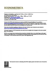
2.3 An exact formalization based on Markov Chains 2.3.1 An absorbing Markov Chain. One interesting way to formalize the problem is to consider it as a sequence of l trials with outcomes X1 , X2 , . . . , Xl . Let each of these outcomes belong to the set {0, 1, . . . , n}, where the outcome i signifies that the i-gram A1 A2 . . . Ai has already occurred. This sequence of trials verifies the following two properties: (i) All the outcomes X1 , X2 , . . . , Xl belong to a finite set of outcomes {0, 1, . . . , n} called the state space of the system. If i is the outcome of the m-th trial (Xm = i), then we say that the system is in state i at the m-th step. In other words, the i-gram A1 A2 . . . Ai has been observed after the m-th word of the document. (ii) The second property is called the Markov property: the outcome of each trial depends at most upon the outcome of the immediately preceding trial, and not upon any other previous outcome. In other words, the future is independent of the past, given the present. This is verified indeed; if we know that we have seen A1 A2 . . . Ai , we only need the probability of Ai+1 to determine the probability that we will see more of the desired n-gram during the next trial. These two properties are sufficient to call the stochastic process we just defined a (finite) Markov chain. The problem can thus be represented by an (n + 1)-states Markov chain M (see figure 1). The state space of the system is {0, 1, . . . , n} where each state, numbered from 0 to n tells how much of the n-gram has already been observed. Presence in state i means that the sequence A1 A2 . . . Ai has been observed. Therefore, Ai+1 . . . An remains to be seen, and the following expected word is Ai+1 . It will be the next word with probability pi+1 , in which case a state transition will occur from i to (i + 1). Ai+1 will not be the following word with probability qi+1 , in which case we will remain in state i. Whenever we reach state n, we can denote the experience a success: the whole n-gram has been observed. The only outgoing transition from state n leads to itself with associated probability 1 (such a state is said to be absorbing).
2.3.2 Stochastic Transition Matrix (in general). Another way to represent this Markov chain is to write its transition matrix.
q1
qn
q2 p1
0
1
p2
pn−1
1 pn
n−1
n
Figure 1: State-transition diagram of the Markov Chain M. For a general finite Markov chain, let pi,j denote the transition probability from state i to state j for 1 ≤ i, j ≤ n. The (one-step) stochastic transition matrix is: 0 1 p1,1 p1,2 . . . p1,n B p2,1 p2,2 . . . p2,n C C P =B @ A ... pn,1 pn,2 . . . pn,n
Theorem 2.1. [6] Let P be the transition matrix of a Markov chain process. Then the m-step transition matrix is equal to the m-th power of P. Furthermore, the entry pi,j (m) in P m is the probability of stepping from state i to state j in exactly m transitions.
2.3.3 Our stochastic transition matrix of interest. For the Markov chain M defined above,the corresponding stochastic transition matrix is the following (n + 1) × (n + 1) square matrix: states 0 0 0 q1 B B0 1 B B . B .. B M= B . B .. B B . @ .. n 0
1 p1
2 0
q2 .. .
p2 .. . .. .
...
...
... ... .. . .. . .. . .. . ...
n−1 ... ..
.
..
.
qn 0
n 0 .. . .. .
1
C C C C C C C 0 C C C pn A 1
Therefore, the probability of the n-gram A1 → A2 → · · · → An to occur in a document of size l is the probability of stepping from state 0 to state n in exactly l transitions. Following Theorem 2.1, this value resides at the intersection of the first row and the last column of the matrix M l : 0
B Ml = B @
m1,1 (l) m2,1 (l)
m1,2 (l) m2,2 (l)
mn+1,1 (l)
mn+1,2 (l)
... ... ... ...
m1,n+1 (l) m2,n+1 (l) mn+1,n+1 (l)
1 C C A
Thus, the result we are seeking can be obtained by raising the matrix M to the power l, and looking at the value in the upper-right corner. In terms of computational complexity, however, one must note that to multiply two (n+1)×(n+1) square matrices, we need to compute (n + 1) multiplications and n additions to calculate each of the (n + 1)2 values composing the resulting matrix. To raise a matrix to the power l means to repeat this operation l − 1 times. The resulting time complexity is then O(ln3 ). One may object that more time-efficient algorithms for matrix multiplication exist. The lowest exponent currently known is by Coppersmith and Winograd: O(n2.376 ) [4]. Such
results are achieved by studying how matrix multiplication depends on bilinear and trilinear combinations of factors. The strong drawback of those techniques is the presence of a constant factor so large that it removes the benefits of the lower exponent for all practical sizes of matrices [8]. For our purpose, the use of such an algorithm is typically more costly than to use the naive O(n3 ) matrix multiplication. Linear algebra techniques, and a careful exploitation of the specificities of the stochastic matrix M will, however, permit to perform a few transformations that will drastically reduce the computational complexity of M l .
2.3.4 The Jordan normal form Definition: A Jordan block Jλ is a square matrix whose elements are zero except for those on the principal diagonal, which are equal to λ, and for those on the first superdiagonal, which are equal to unity. Thus: 0
B B Jλ = B B @
λ
1
0
λ 0
..
.
..
.
1
C C C. C 1 A λ
Theorem 2.2. (Jordan normal form) [11] If A is a general square matrix, then there exists an invertible matrix S such that 1 0 J1 0 C B .. J = S −1 AS = @ A, . 0
to express vj+1 in terms of vj , and therefore in terms of v1 . That is, for 1 ≤ j ≤ n : vj+1 =
e − qj (e − qj ) . . . (e − q1 ) vj = v1 . pj pj . . . p1
In general (for all the qi ’s), v1 can be chosen freely to have any non null value. This choice will uniquely determine all the values of V . Since the general form of the eigenvectors corresponding to any eigenvalue of M is V = [v1 , v2 , . . . , vn+1 ], where all the values can be determined uniquely by the free choice of v1 , it is clear that no two such eigenvectors can be linearly independent. Hence, one and only one eigenvector corresponds to each eigenvalue of M . Following theorem 2.2, this means that there is a single Jordan block for each eigenvalue of M , whose size equals to the order of algebraic multiplicity of the eigenvalue, that is, its number of occurrences in the principal diagonal of M . In other words, there is a distinct Jordan block for every distinct qi (and its size equals the number of occurrences of qi in the main diagonal of M ), plus a block of size 1 for the eigenvalue 1. Therefore we can write 0 1 Je1 0 B C .. C, J = S −1 M S = B . @ A 0 J eq where the Jei are ni × ni Jordan blocks, corresponding to the distinct eigenvalues of M . Following general properties of the Jordan normal form, we have
Jk
0
where the Ji are ni × ni Jordan blocks. The same eigenvalues may occur in different blocks, but the number of distinct blocks corresponding to a given eigenvalue is equal to the number of eigenvectors corresponding to that eigenvalue and forming an independent set. The number k and the set of numbers n1 , . . . , nk are uniquely determined by A. In the following subsection we will demonstrate that M is a matrix such that there exists only one block for each eigenvalue.
2.3.4.1 Uniqueness of the Jordan block corresponding to any given eigenvalue of M . Theorem 2.3. For the matrix M , no two eigenvectors corresponding to the same eigenvalue can be linearly independent. Proof. Because M is triangular, its characteristic polynomial is the product of the diagonals of (λIn+1 − M ): f (λ) = (λ − q1 )(λ − q2 ) . . . (λ − qn )(λ − 1). The eigenvalues of M are the solutions of the equation f (λ) = 0. Therefore, they are the distinct qi ’s, and 1. Now let us show that whatever the order of multiplicity of such an eigenvalue (how many times it occurs in the set {q1 , . . . , qn , 1}), it has only one associated eigenvector. The eigenvectors associated to a given eigenvalue e are defined as the non null solutions of the equation M · V = e · V . If we write the coordinates of V as [v1 , v2 , . . . , vn+1 ], we can observe that M · V = e · V results in a system of (n + 1) equations, where, for 1 ≤ j ≤ n, the j-th equation permits
B B Jl = B @
Also,
M
l
=
Jel1
z`
SJS
−1
z`
.. 0
. Jelq
1
C C C. A
l times }| ´ ´ ` ` ´{ · SJS −1 . . . SJS −1 −1
(l − 1) times ` −1 }| ´ ` ´ { · S · J · S · S · J . . . S −1 · S · J ·S −1 ´
=
S·J · S
=
l times z }| { S · J · J . . . J ·S −1
=
0
S · J l · S −1 .
Therefore, by multiplying the first row of S by J l , and multiplying the resulting vector by the last column of S −1 , we do obtain the upper right value of M l , that is, the probability of the n-gram (A1 → · · · → An ) to appear in a document of size l.
2.3.4.2 Calculating powers of a Jordan block. As mentioned above, to raise J to the power l, we can simply write a direct sum of the Jordan blocks raised to the power l. In this section, we will show how to compute Jeli for a Jordan block Jei . Let us define Dei and Nei such that Jei = Dei + Nei , where Dei contains only the principal diagonal of Jei , and Nei only its first superdiagonal. That is,
qa=2/3 Dei
0
B B =B @
0
ei ei ..
.
0
0
1
ei
B C B C C and Nei = B @ A
0
1
0 ..
.
0
1
C C C. 1 A 0
Observing that Nei Dei = Dei Nei , we can use the binomial theorem: ! l X l l l Neki Del−k Jei = (Dei + Nei ) = i k
k=0
Hence, to calculate one can compute the powers of Dei and Nei from 0 to l, which is a fairly simple task. The power of a diagonal matrix is easy to compute, as it is another diagonal matrix where each term of the original matrix is raised to the same power as the matrix. Deji is thus identical to Dei , except that the main diagonal is filled with the value eji instead of ei . To compute Neki is even simpler. Each multiplication of a power of Nei by Nei results in shifting the non-null diagonal one row upwards. The result of Neki Deji resembles Neji , except that the ones on the only non-null diagonal (the j-th superdiagonal) are replaced by the value of the main diagonal of Deji , that is eji . Therefore, we have: 0 1 0 el−k 0 i B C .. B C . B C k l−k N ei Dei = B l−k C . ei B C @ A
..
.
2.3.5 Conclusion
´
i +1 · el−n i .. ` l ´ . l−k · ei k .. ` l ´. l · ei 0
The probability of the n-gram (A1 → · · · → An ) in a document of size l can be obtained as the upper-right value in the matrix M l such that:
Ml
The state-transition diagram of the Markov Chain corresponding to the bigram A → B has only three states (figure 2). The corresponding transition matrix is: 0 2 1 1 0 3 3 2 1 Mre = @ 0 3 3 A . 0 0 1
Following Theorem 2.2 on the Jordan normal form, there exists an invertible matrix Sre such that 1 0 J 0 2 −1 A, Mre Sre = @ 3 Jre = Sre 0 J1 where J1 is a block of size 1, and J 2 a block of size 2 since 3
qa = qb = 32 . We can actually write Jre as: 0 2 1 1 0 3 Jre = @ 0 23 0 A . 0 0 1
to a distinct diagonal, easily written as:
l ni −1
0
B B = SJ l S −1 = S B @
Jel1
0 ..
0
. Jelq
1
C C −1 CS , A
2 seen:AB
2.3.6 Running Example.
0
`
seen:A
where the Jeli blocks are as described above, while S and S are obtained through the Jordan Normal Form theorem (Theorem 2.2). We actually only need the first row of S and the last column of S −1 , as we are not interested in the whole matrix M l but in its upper-right value only. In the next subsection we will calculate the worst case time complexity of the technique that we just presented. Before that, let us return to the running example presented in subsection 2.1.2.
Jeli ,
... .. .
seen: o/
pb=1/3
1
−1
Because Nei is nilpotent (Neki = 0, ∀k ≥ ni ), we can shorten the summation to: ! ni −1 X l l l Neki Del−k Jei = (Dei + Nei ) = i k
Since each value P of `k ´corresponds is the summation lk=0 kl Neki Del−k i ! l X l Neki Del−k Jeli = i k k=0 ` l ´ l−k 0 `l´ l · ei · ei . . . k 0 B .. B . B `l´ l B = B · ei 0 B B @ 0
pa=1/3
1
Figure 2: State-transition diagram of the Markov Chain corresponding to our running example.
k=0
0
0
qb=2/3
1
C C C C C. C C A
Since we seek the probability of the bigram A → B in a 3 document of size 3, we need to calculate Jre : 0 ` 3´ 2 3 ` 3´ 2 2 1 08 1 4 ( 3 ) ` 1´ ( 3 ) 0 0 0 27 3 3 8 3 = @ 0 Jre 0A . ( 32 )3 0A = @ 0 27 0 0 0 1 0 0 1
In the next subsection, we will give further details as to the practical computation of Sre and the last column of −1 . For now, let us simply assume they were its inverse Sre calculated, and we can thus obtain the probability of the bigram AB in a document of length 3 as: last col. of S −1 z }| 1{ 0 1 −1 0 @− 1 A 0A 3 1 1
1st row of S 0 8 4 z }| { 27 3 8 P (A → B, 3) = (1 0 1) @ 0 27 0 0 7 . = 27 Our technique indeed obtains the right result. But how efficiently is it obtained? We overview an answer to this question in the following subsection.
2.4 Algorithmic Complexity The process of calculating the probability of occurrence of an n-gram in a document of size l consists of two main phases: calculating J l , and computing the transformation matrix S and its inverse S −1 . Below, we will study the worst case time complexity, but it is interesting to observe that in practice, for a corpus big enough, the number of words equally-weighed should be small. This is especially true since, following Zipf’s law, infrequent words are most likely to have equal weights, and they precisely are often pruned during preprocessing. The following complexity analysis might be easier to follow, if studied together with the general formulas of M l and the Jordan blocks as presented in the conclusion of subsection 2.3 (subsection 2.3.5).
2.4.1 Time complexity of the J l calculation Observing that each block Jil contains P exactly ni distinct values, we can see that J l contains 1≤k≤q nk = n + 1 distinct values. Those (n + 1) values are (n + 1) multiplications of a binomial coefficient by a power of an eigenvalue. The computation of the powers between 0 and l of each eigenvalue is evidently achieved in O(lq), because each of the q distinct eigenvalues needs to be multiplied by itself l times. For every Jordan J`il , the´binomial coefficients to be ´ ` l ´ `block l computed are: 0 , 1 , . . . , nil−1 . For the whole matrix J l , ` ´ we thus need to calculate kl where 0 ≤ k ≤ maxblock and ` l ´ ` l ´ l−j = j j+1 , and maxblock = maxqi=1 ni . Observing that j+1 ` l ´ `´ thus, that j+1 can be computed from jl in a constant ` ´ number of operations, we see that the set { kl | 1 ≤ k ≤ maxblock } can be computed in O(maxblock ). If l < n, the probability of occurrence of the n-gram in l is 0, since the n-gram is longer than the document. Therefore, the current algorithm is only used when l ≥ n ≥ maxblock . We can therefore conclude that the time complexity of the computation of J l is O(lq).
2.4.2 Calculating the transformation matrix S Following general results of linear algebra [11], the (n + 1) × (n + 1) transformation matrix S can be written as: ˆ ˜ S = S1 S2 . . . S q ,
where each Si is an ni × (n + 1) matrix corresponding ˜ to the ˆ eigenvalue ei , and such that Si = vi,1 vi,2 . . . vi,ni , where:
• vi,1 is an eigenvector associated with ei , thus such that, M vi,1 = ei vi,1 , and • vi,j , for all j = 2 . . . ni , is a solution to the equation M vi,j = ei vi,j + vi,j−1 .
The vectors vi,1 vi,2 . . . vi,ni are sometimes called generalized eigenvectors of ei . We have already seen in section 2.3.4, that the first coordinate of each eigenvector can be assigned freely, and that every other coordinate can be expressed in function of its immediately preceding coordinate. Therefore it takes a constant number of operations to calculate the value of each coordinate of an eigenvector, and each eigenvector can be computed in O(n). It is equally provable that the generalized eigenvectors can be expressed and calculated in a constant number of operations. Following this fact, each column of S can be computed in O(n), and thus the whole matrix S in O(n2 ).
2.4.3 The inversion of S The general inversion of an (n + 1) × (n + 1) matrix can be done in O(n3 ) through Gaussian elimination. To calculate only the last column of S −1 does not help, since the resulting system of (n + 1) equations still requires O(n3 ) operations to be solved by Gaussian elimination. However, some specificities of our problem will again permit an improvement over this general complexity. When calculating the similarity matrix S, we can ensure that S is a column permutation of an upper-triangular matrix. It is therefore possible to calculate the last column of S −1 by solving a triangular system of linear equations through a backward substitution mechanism. The computation of the last column of S −1 is thus achieved in O(n2 ).
2.4.4 Conclusion To obtain the final result, the probability of occurrence of the n-gram in a document of size l, it remains to multiply the first row of S by J l , and the resulting vector by the last column of S −1 . The second operation takes (n + 1) multiplications and n additions. It is thus O(n). The general multiplication of a vector of size (n + 1) by an (n + 1) × (n + 1) square matrix takes (n + 1) multiplications and n additions for each of the (n+1) values of the resulting vector. This is thus O(n2 ). However, we can use yet another trick to improve this complexity. When we calculated the matrix S, we could assign the first row values of each column vector freely. We did it in such a way that the only non-null values on the first row of S are unity, and that they occur on the q eigenvector columns (these same choices ensured that S is a column permutation of an upper-triangular matrix). Therefore, to multiply the first row of S by a column vector simply consists in the addition of the q terms of index equal to the index of the eigenvectors in S. That operation of order O(q) needs to be repeated for each column of J l . The multiplication of the first row of S by J l is thus O(nq). The worst case time complexity of the computation of the probability of occurrence of an n-gram in a document of size l is finally max{O(lq), O(n2 )}. Since our problem of interest is limited to l ≥ n (otherwise the probability of occurrence is 0), an upper bound of the complexity for computing the probability of occurrence of an n-gram in a document of size l is O(ln). This is clearly better than directly raising M to the power l, which is O(ln3 ).
3. EXPECTED DOCUMENT FREQUENCY OF A WORD SEQUENCE Now that we have defined a formula to calculate the probability of occurrence of an n-gram in a document of size l, we can use it to calculate the expected document frequency of the n-gram in the whole document collection D. Assuming the documents are mutually independent, the expected frequency in the document collection is the sum of the probabilities of occurrence in each document: X Exp df (A1 → . . . An , D) = p(A1 → . . . An , |d|), d∈D
where |d| stands for the number of word occurrences in the document d. Naive Computational Complexity. We can compute the probability of an n-gram to occur in a document in
O(ln). A separate computation and summation of the values for each document can thus be computed in O(|D|ln), where |D| stands for the number of documents in D. In practice, we can improve the computational efficiency by counting the number of documents of same length and multiplying this number by the probability of occurrence of the n-gram in a document of that size, rather than reprocessing and summing up the same probability for each document of equal size. But as we are currently considering the worst case time complexity of the algorithm, we are facing the worst case situation in which every document has a distinct length. Better Computational Complexity. We can achieve better complexity by summarizing everything we need to calculate and organizing the computation in a sensible way. Let L = maxd∈D |d| be the size of the longest document in the collection. We first need to raise the Jordan matrix J to the power of every distinct document length, and then to multiply the (at worst) |D| distinct matrices by the first row of S and the resulting vectors by the last column of its inverse S −1 . The matrix S and the last column of S −1 need to be computed only once, and as we have seen previously, this is achieved in O(n2 ), whereas the |D| multiplications by the first row of S are done in O(|D|nq). It now remains to find the computational complexity of the various powers of J. We must first raise each eigenvalue ei to the power L, which is an O(Lq) process. For each document d ∈ D, we obtain all the terms of J |d| by (n + 1) multiplications of powers of eigenvalues by a set of combinatorial coefficients computed in O(maxblock ). The total number of such multiplications is thus O(|D|n), an upper bound for the computation of all combinatorial coefficients. The worst case time complexity for computing the set { J |d| | d ∈ D}, is thus max{O(|D|n), O(Lq)}. Finally, the computational complexity for calculating the expected frequency of an n-gram in a document collection D is max{O(|D|nq), O(Lq)}, where q is the number of words in the n-gram having a distinct probability of occurrence, and L is the size of the longest document in the collection. The improvement is considerable compared to the naive technique’s O(|D|ln3 ).
4.
DIRECT EVALUATION OF LEXICAL COHESIVE RELATIONS
The evaluation of lexical cohesion is a difficult problem. Attempts of direct evaluation are rare, simply due to the subjectivity of any human assessment and due to the wide acceptance that we first need to know what we want to do with a lexical unit before being able to decide whether or not it is relevant for that purpose. A common application of research in lexical cohesion is lexicography, where the evaluation is carried out by human experts who simply look at phrases to assess them as good or bad. This process permits to score the extraction process with highly subjective measures of precision and recall. However, a linguist interested in the different forms and uses of the auxiliary “to be” will have a different view of what is an interesting phrase than a lexicographer. What a human expert judges as uninteresting may be highly relevant to another. Hence, most evaluation has been indirect, through question answering, topic segmentation, text summarization, and
passage or document retrieval [12]. To pick the last case, such an evaluation consists in trying to figure out which are the phrases that permit to improve the relevance of the list of documents returned. A weakness of indirect evaluation is that it hardly shows whether an improvement is due to the quality of the phrases, or to the quality of the technique used to exploit them. There is a need to fill the lack of a general purpose direct evaluation technique, one where no subjectivity or knowledge of the domain of application will interfere. Our technique permits exactly that, and this section will show how.
4.1 Hypothesis testing A general approach to estimate the interestingness of a set of events is to measure their statistical significance. In other words, by evaluating the validity of the assumption that an event occurs only by chance (the null hypothesis), we can decide whether the occurrence of that event is interesting or not. If a frequent occurrence of a multi-word unit was to be expected, it is less interesting than if it comes as a surprise. To estimate the quality of the assumption that an n-gram occurs by chance, we need to compare its (by chance) expected frequency and its observed frequency. There exists a number of statistical tests, extensively described in statistics textbooks, even so in the specific context of natural language processing [9]. In this paper, we will base our experiments on the t-test: t=
Obs df (A1 → . . . An , D) − Exp df (A1 → . . . An , D) p |D|Obs DF (A1 → . . . An )
4.2 Example of non-contiguous lexical units: MFS Maximal Frequent Sequences (MFS) [1] are word sequences built with an unlimited gap, no stoplist, no POS analysis and no linguistic filtering. They are defined by two characteristics: • A sequence is said to be frequent if its document frequency is higher than a given threshold. • A sequence is maximal, if there exists no other frequent sequence that contains it. Thus, MFSs correspond very well to our technique, since the extraction algorithm provides each extracted MFS with its document frequency. To compare the observed frequency of MFSs to their expected frequency is thus especially meaningful, and it will permit to rank a set of MFSs with respect to their statistical significance.
4.3 Experiments 4.3.1 Corpus For experiments we used the publicly available Reuters21578 newswire collection 1 , which originally contains about 19, 000 non-empty documents. We split the data into 106, 325 sentences. The average size of a sentence is 26 word occurrences, while the longest sentence contains 260. Using a minimum frequency threshold of 10, we extracted 4, 855 MFSs, distributed in 4, 038 2-grams, 604 3-grams, 141 4-grams, and so on. The longest sequences had 10 words. 1
http://www.daviddlewis.com/resources/textcollections/reuters21578
t-test 0.03109 0.02824 0.02741 0.02666 0.02485
n-gram los angeles kiichi miyazawa kidder peabody morgan guaranty latin america
expected 0.08085 0.09455 0.04997 0.20726 0.65666
observed 103 85 80 76 67
Table 1: Overall Best 5 MFSs t-test 9.6973-03 9.6972-03 9.6969-03 9.6968-03 9.6968-03 8.2981-03 8.2896-03 8.2868-03 8.2585-03 8.2105-03
n-gram het comite piper jaffray wildlife refuge tate lyle g.d searle pacific security present intervention go go bills holdings cents barrel
expected 0.6430-03 0.8184-03 0.0522-03 0.1458-03 0.1691-03 1.4434 1.4521 1.4551 1.4843 1.5337
observed 10 10 10 10 10 10 10 10 10 10
Table 2: The t-test applied to the 5 best and worst bigrams of frequency 10
The expected document frequency and the t-test of all the MFSs were computed in 31.425 seconds on a laptop with a 1.40 Ghz processor and 512Mb of RAM. We used an implementation of a simplified version of the algorithm that does not make use of all the improvements presented in this paper.
4.3.2 Results Table 1 shows the overall best-ranked MFSs. In Table 2, we can compare the best-ranked bigrams of frequency 10 to their last-ranked counterparts, noticing a difference in quality that observed frequency alone does not reveal. It is important to note that our technique permits to rank longer n-grams amongst pairs. For example, the best-ranked n-gram of size higher than 2 lies in the 10th position: “chancellor exchequer nigel lawson” with t-test value 0.023153, observed frequency 57, and expected frequency 0.2052e − 07. In contrast to this high-ranked 4-gram, the last-ranked n-gram of size 4 occupies the 3, 508th position: “issuing indicated par europe” with t-test value 0.009698, observed frequency 10, and expected frequency 22.25e − 07.
5.
CONCLUSION
We presented a novel technique for calculating the probability and expected document frequency of any given noncontiguous lexical cohesive relation. We found a Markov representation for the problem and exploited the specificities of that representation to obtain a low computational complexity. We further described a method that compares observed and expected document frequencies through a statistical test as a way to give a direct numerical evaluation of the intrinsic quality of a multi-word unit (or of a set of multi-word units). This technique does not require work of a human expert, and it is fully language- and application-independent. It is generally accepted that, in English, two words at a
distance five or more are not connected. We can attempt to deal with this by using short documents, for example sentences, or even comma-separated units. A weakness that our approach shares with most language models is the assumption that terms occur independently from each other. In the future, we hope to present more advanced Markov representations that will permit to account for term dependency.
6. REFERENCES [1] H. Ahonen-Myka and A. Doucet. Data mining meets collocations discovery. In print, pages 1–10. CSLI Publications, Center for the Study of Language and Information, University of Stanford, 2005. [2] Y. Choueka, T. Klein, and E. Neuwitz. Automatic retrieval of frequent idiomatic and collocational expressions in a large corpus. Journal for Literary and Linguistic computing, 4:34–38, 1983. [3] K. W. Church and P. Hanks. Word association norms, mutual information, and lexicography. Computational Linguistics, 16(1):22–29, 1990. [4] D. Coppersmith and S. Winograd. Matrix multiplication via arithmetic progressions. In STOC ’87: Proceedings of the nineteenth annual ACM conference on Theory of computing, pages 1–6, 1987. [5] G. Dias. Multiword unit hybrid extraction. In Workshop on Multiword Expressions of the 41st ACL meeting. Sapporo. Japan., 2003. [6] W. Feller. An Introduction to Probability Theory and Its Applications, volume 1. Wiley Publications, third edition, 1968. [7] K. T. Frantzi, S. Ananiadou, and J. ichi Tsujii. The c-value/nc-value method of automatic recognition for multi-word terms. In ECDL ’98: Proceedings of the Second European Conference on Research and Advanced Technology for Digital Libraries, pages 585–604. Springer-Verlag, 1998. [8] R. A. Horn and C. R. Johnson. Topics in matrix analysis. Cambridge University Press, New York, NY, USA, 1994. [9] C. D. Manning and H. Sch¨ utze. Foundations of Statistical Natural Language Processing. MIT Press, Cambridge MA, second edition, 1999. [10] M. Mitra, C. Buckley, A. Singhal, and C. Cardie. An analysis of statistical and syntactic phrases. In Proceedings of RIAO97, Computer-Assisted Information Searching on the Internet, pages 200–214, 1987. [11] B. Noble and J. W. Daniel. Applied Linear Algebra, pages 361–367. Prentice Hall, second edition, 1977. [12] V. O. The role of multi-word units in interactive information retrieval. In Proceedings of the 27th European Conference on Information Retrieval, Santiago de Compostela, Spain, pages 403–420, 2005. [13] F. Smadja. Retrieving collocations from text: Xtract. Journal of Computational Linguistics, 19:143–177, 1993. [14] T. Tanaka, A. Villavicencio, F. Bond, and A. Korhonen, editors. Second ACL Workshop on Multiword Expressions: Integrating Processing, 2004.