A methodology for comparing classifiers that allow the ...

A methodology for comparing classifiers that allow the control of bias Anton Zamolotskikh

Sarah Jane Delany

University of Dublin, Trinity College Dublin 2, Ireland

Dublin Institute of Technology Kevin Street, Dublin 8, Ireland

[email protected] ABSTRACT

This paper presents False Positive-Critical Classifiers Comparison a new technique for pairwise comparison of classifiers that allow the control of bias. An evaluation of Na¨ıve Bayes, k-Nearest Neighbour and Support Vector Machine classifiers has been carried out on five datasets containing unsolicited and legitimate e-mail messages to confirm the advantage of the technique over Receiver Operating Characteristic curves. The evaluation results suggest that the technique may be useful for choosing the better classifier when the ROC curves do not show comprehensive differences, as well as to prove that the difference between two classifiers is not significant, when ROC suggests that it might be. Spam filtering is a typical application for such a comparison tool, as it requires a classifier to be biased toward negative prediction and to have some upper limit on the rate of false positives. Finally the particular evaluation summary is presented, which confirms that Support Vector Machines outperform other methods in most cases, while the Na¨ıve Bayes classifier works well in a narrow, but relevant range of false positive rate.

1.

Padraig Cunningham ´

University of Dublin, Trinity College Dublin 2, Ireland [email protected]

INTRODUCTION

A requirement for a classifier to be biased towards a particular prediction arises in situations when different misclassification errors have different costs. A typical example of such a situation is spam filtering, although there are other areas where the control of bias can be useful, such as the detection of emergency situations in information and industrial systems, data mining problems etc. Thus an evaluation of classifiers that allow the control of bias is an important problem. The experimental part of our work covers the application of machine learning to spam filtering. The amount of spam received by email users worldwide dramatically exceeds the amount of legitimate mail and it is growing. As users are able to contribute to the classification of email messages, a natural supervised machine learning problem arises, i.e. to

[email protected]

build a classifier based on a training set of messages labeled by a human. The accuracy of a classifier is not the only important feature in the spam filtering context, as the misclassification of spam as non-spam is much less important than the misclassification of legitimate mail as spam. If the former may result in the increase of unwanted mail a user receives, the latter could cause important mail to go missing. For this reason, the classifier must be biased towards negative (nonspam) prediction to reduce the rate of false positives, as it is stressed in the work of Androutsopoulos et al [1] and Hidalgo et al [7]. The Receiver Operating Characteristic (ROC) [12] curve analysis and comparison of the area under the curve (AUC) [2] are common evaluation techniques. The disadvantage of ROC is that it can suggest that one classifier performs better than another which cannot be confirmed with statistical significance. On the other hand, a statistically significant advantage of one classifier over another may show up as a very small difference between corresponding ROC curves. The paper presents False Positive-Critical Classifier Comparison (FP-C3 ), a new technique tailored to a situation which requires classification to be biased towards or away from certain predictions. The technique also uses a statistical significance test, in this case we have used McNemar’s test [5]. We compare three classifiers using the FP-C3 technique, each of which can be biased towards negative or positive prediction. The classifiers include the k nearest neighbour (k-NN) algorithm [1], Na¨ıve-Bayes (NB) [10] and Support Vector Machines (SVM) [3]. The remainder of the paper is organised as follows. Section 2 discusses the classifiers and datasets used in the evaluation, as well as the traditional ROC curve analysis method. Section 3 describes the FP-C3 technique we propose and Section 4 discusses examples of the application of both ROC and FP-C3 analysis on experimental data. Section 5 presents our experimental results and highlights the different assessment of ROC analysis and the new evaluation technique on the same results. Finally Section 6 presents our conclusions.

2. COMPARING CLASSIFIERS Permission to make digital or hard copies of all or part of this work for personal or classroom use is granted without fee provided that copies are not made or distributed for profit or commercial advantage and that copies bear this notice and the full citation on the first page. To copy otherwise, to republish, to post on servers or to redistribute to lists, requires prior specific permission and/or a fee. SAC’06 April 23-27, 2006, Dijon, France Copyright 2006 ACM 1-59593-108-2/06/0004 ...$5.00.

The problem of selecting the classifier which performs best on some particular test set can be solved in different ways that depend on the criteria of performance. The most basic criterion is accuracy, i.e. the rate of correctly classified cases. One of the most common ways to measure the accuracy of a classifier on the particular labeled data set is to perform N-fold cross-validation. The classifier is applied N times to

the dataset, training on NN−1 of samples and then classifying the remaining N1 samples as a test set. Each time different samples are selected as a test set, so at the end all samples of the original data set have been classified, the predictions for the samples can be compared with their known labels (solutions) and the accuracy can be calculated. Accuracy is not the only way to assess and compare classifiers. First of all, achieving higher accuracy may be less important than achieving lower number of misclassified samples of a particular class. In the spam filtering scenario, for example, a minimisation of the amount of legitimate messages classified as spam is a priority, while the overall accuracy is less important. If we consider spam messages to be members of a ”positive” class, the rate of such misclassification is called the rate of false positive errors (FP rate). It is also important to note that an advantage in accuracy of one classifier in comparison to another detected on some particular dataset may not be statistically significant and may not allow to make general conclusion about this advantage based on such evaluation. This problem is addressed by statistical significance tests, such as t-test and McNemar’s test. Classifiers, which allow adjusting the bias toward either negative or positive prediction, may perform differently in terms of accuracy and FP rate depending on the particular bias applied. So the FP rate can be reduced appropriately by decreasing the accuracy or vice versa. Comparing two such classifiers for all possible values of bias is addressed by ROC curves (see Section 2.3).

2.1

Classifiers

This section describes the three different classification algorithms that have been used for the evaluation; the k-NN classifier, the NB classifier and the SVM. Each classifier supports the application of different levels of bias towards negative or positive prediction.

2.1.1 k Nearest Neighbour The k-NN classifier returns the k most similar cases to the query case from a case-base of training data. The prediction is determined from these k neighbours using a distanceweighted voting algorithm. Assuming each training case is represented as a vector of features ei = {f1 , . . . , fn }, the classification for query case xq , over the k nearest neighbours x1 , . . . xk is given in Equation 1 where 1(a, b) = 1 if a = b, 1(a, b) = 0 if a 6= b , wj is given in Equation 2, fi (xj ) is the value of feature i in case xj and cj is the classification of neighbour xj .

ckN N = argmax ci ∈C

wj =

n X

k X

wj 1(cj , ci )

(1)

j=1

!2

|fm (xq ) − fm (xj )|

(2)

m=1

To apply a bias to the classifier the score for the positive and negative classifications are normalised. By comparing the resulting normalised score for a specific classification to a threshold that can take any value in the range of possible classification scores, i.e. between zero and one, the classifier can be biased towards or away from the specific classification. For instance, the classifier can be strongly biased away

from a positive prediction by setting the threshold value to 0.9, say, requiring that the the normalised score for the positive classification is greater than this threshold value before the classification returned is positive. A threshold value of 0.5 corresponds to a majority vote scenario. Two types of k-NN classifier have been used in this evaluation. The first uses the full training set of cases. The second is a k-NN classifier which applies a case-based editing technique called Competence Based Editing (CBE) to the training data before classifying the test cases. CBE was developed for the spam filtering domain to identify and remove noisy and redundant cases from a case-base of spam and legitimate emails. It has been shown to increase the generalisation accuracy of a case-base in this domain [4].

2.1.2

Na¨ıve Bayes

NB is a probabilistic classifier that can handle high dimension data which can be a problem with alternative machine learning techniques. It is ‘na¨ıve’ in the sense that it assumes that the features are independent. The classification returned from a NB classifier applied to cases represented by binary features for a query example xq is given in Equation 3 cN B = argmax P (ci ) ci ∈C

n Y

P (fj (xq )|ci )

(3)

j

The conditional probabilities can be estimated by P (fi (xq )|cj ) = nij /nj where nij is the number of times that feature fi occurs in those training examples with classification cj and nj is the number of training examples with classification cj . This provides a good estimate of the probability in many situations but in situations where nij is very small or even equal to zero this probability will dominate, resulting in an overall zero probability. A solution to this is to incorporate a small-sample correction into all probabilities called the Laplace correction [9]. The corrected probability estimate is given by Equation 4, where nki is the number of values for attribute ai . Kohavi et al. [8] suggest a value of f = 1/m where m is equal to the number of training documents. P (fi (xq )|cj ) =

nij + f nj + f nki

(4)

In a similar way to the k-NN classifier, the NB classifier can be biased towards a positive or negative classification by apply a decision threshold to the classification score.

2.1.3

Support Vector Machine

A Support Vector Machine is a linear maximal margin 2-class classifier. The latter is a solution to an optimisation problem of finding the hyperplane in the feature space, which maintains the largest margin between the members of one class and the members of the other closest to the hyperplane. These closest members are support vectors, as they define the hyperplane. As the original feature space is not alway linearly separable it can be projected into an artificially constructed hyperspace of higher dimensionality. The solution to the optimisation problem in the SVM uses cases only in the form of the dot product of each pair of samples in the constructed feature space. That allows calculating the dot product in the constructed hyper-space using values of the original features, without the explicit calculation of the constructed features. Such a dot product is called

a kernel function. In the case of text, the dimensionality of the original feature space is usually high enough, allowing the simple dot product to be used as a kernel function. The soft-margin SVM [11] used in this evaluation allows some cases from the training set to be within the margin or even on the “wrong” side of the hyperplane. Such an approach makes SVM less sensitive to noise. The degree to which such errors are allowed is determined by an error cost. The soft-margin SVM can be biased by either applying different error costs to representatives of different classes, or by applying a non-zero threshold to its real-valued output. The latter approach has been used in this evaluation, as it gives better control over the ratio of true positives to false positives, which is a useful feature in applications of SVM to such domains as spam filtering [6].

Having plotted ROC curves for two or more classifiers, it is possible to detect the ranges of FP rates in which one curve is higher than another and conclude that the classifier corresponding to the higher curve performs better in terms of TP rate for these ranges of FP rates. Our evaluation shows that such a conclusion may not, in fact, be statistically supported (see Sections 4 and 5). The area under the curve (AUC) has a statistical meaning, as it reflects the probability of the classifier predicting a higher score for a positive sample than for a negative one. Using this metric, two classifiers can be compared without the application of any particular threshold of judgment. The problem with this method is that it does not give any information on a particular range of FP rates.

2.2

McNemar’s approximate statistical significance test [5] is used to compare two classifiers at a particular value of bias. To determine if one classifier (C1 ) significantly outperforms the other (C2 ), the χ2 statistic is calculated as follows:

Datasets

The datasets were derived from two corpora of email collected by two individuals over the period of one year. Datasets 1 and 2 were extracted from the first corpus and datasets 3,4 and 5 from the second. Each included 500 spam emails and 500 legitimate emails, received consecutively, so each datasets covers a specific period of time. The emails were not altered to remove HTML tags and no stop word removal or stemming was performed on the text. A subset of the header information from the emails was used, including subject text, and the text from the to: and cc: fields. Each email was reduced to a vector of features ei = {f1 , f2 , . . . , fn } where each feature fi is represented as binary. If the feature exists in the email then fi = 1 otherwise fi = 0. Features were identified by tokenising the email into words and characters and by including certain statistics such as the proportion of uppercase, lowercase, punctuation and white space characters. No domain specific information was included.

2.3

Receiver Operating Characteristic Curves

The Receiver Operation Characteristic curve was originally developed in radar technologies, emerging after WWII. Later it was applied to medical experiments and drug testing. Swets [12] first proposed using the ROC curve to compare classifiers and it has now become a widely accepted way to assess classifiers which allow bias towards either negative or positive prediction. The ROC is plotted in two coordinates; the FP rate on the x axis and the true positive (TP) rate on the y axis. Adjusting the classifier to produce different FP rates allows the depiction of an ROC curve, as each FP rate level corresponds to some TP rate level. It is expected that the TP rate rises as the FP rate does, so the curve monotonously increases from the bottom left to the top right of the chart. The bottom left-hand corner represents the classifier which predicts zero true positives and zero false positives, which means that it always makes a negative prediction. The top right-hand corner represents a classifier which predicts 100% true positives and 100% false positives, which means that it always makes a positive prediction. The diagonal line between these two corners represents the “random” classifier, which does not take any features into consideration when making predictions, so it is expected that any useful classifier would be represented by a curve above this diagonal. The top left-hand corner represents an ideal classifier, which predicts 100% true positives and no false positives, i.e. does not make any mistakes.

2.4

McNemar’s Test

(|n01 − n10 | − 1)2 (5) n01 + n10 where n01 is a number of cases misclassified by C1 and classified correctly by C2 , and n10 is a number of cases misclassified by C2 and classified correctly by C1 . If the null hypothesis, which states that one classifier performs no better than the other, is correct then the probability of χ2 being greater than χ21,0.95 = 3.841459 is lower than 5%. So if the calculated statistic (χ2 ) is greater than that, we may reject the null hypothesis, assuming that one classifier performs better than the other. χ2 =

3.

THE FP-C3 TECHNIQUE

Addressing the disadvantages of ROC curves for FP-critical classifiers, we introduce FP-C3 a new technique for comparing such classifiers based on a statistical significance test. In this evaluation we use McNemar’s test (see section 2.4) but the FP-C3 technique may use any statistical test. FPC3 was developed specifically for spam filtering to allow the comparison of classifiers in an FP-critical domain but may be applied outside this domain. The requirements of a FP-critical classifier can be expressed as follows: (i) The classifier’s FP rate must stay under some particular threshold, otherwise the classifier is not suitable irre-

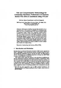
Figure 1: FP-C3 construction technique illustrated using ROC curves.

spective of any other characteristics. (ii) A classifier is considered to be better if it produces a significantly higher TP rate while maintaining (i) above. (iii) The advantage of the better classifier can be measured as the maximum difference in FP rates. The motivation behind FP-C3 is to illustrate when performance advantages suggested by ROC analysis are statistically significant. This is illustrated in Figure 1 which shows the FP margin between two classifiers for which the TP benefit is statistically significant. The FP-C3 chart for two classifiers C1 and C2 depicts the FP rate of the classifier suspected to be worse (C1 , say) on C2 the x axis and the advantage AdvC (F PC1 ) of the suspected 1 better classifier C2 over C1 on the y axis (see equation 6). C2 AdvC (F PC1 ) = 1

F PC1 min

sig

T PC2 > T PC1

F PC2

−1

(6)

sig

where T PC2 > T PC1 means that one rate is significantly better than another in terms of the statistical significance test used. The FP advantage figure plotted on the y axis represents the percentage increase in FPs produced by the losing classifier over the winning classifier when the winning classifier has a significantly higher TP rate. An advantage of zero means that for a FP rate no higher than F PC1 , C2 has no significantly better TP rate than C1 . An advantage equal to 100% means that for the specified FP rate, C2 has a significantly higher TP rate than C1 and C1 ’s FP rate is twice as high as C2 ’s. As we show in the Examples section, FP-C3 also allows us to identify significant differences between classifiers when they are not clearly visible on the ROC curves and also to show that one classifier is not actually better than another when ROC curve analysis suggests that it might be. Two FP-C3 charts can be constructed for each pair of classifiers C1 and C2 ; the first assumes that C1 is worse than C2 and the second which assumes C2 is worse than C1 . We propose to plot both curves on a single chart, one in the positive halfplane and the other reversed in the negative halfplane. The resulting chart will clearly highlight the ranges of FP values for which one classifier gives significant advantantage over another.

4.

EVALUATION EXAMPLES

To illustrate the FP-C3 technique on real results let us consider several examples from the evaluation carried out. The evaluation results for dataset 5 provide an opportunity to illustrate the FP-C3 analysis in conjunction with ROC curve analysis. Figure 4 shows ROC curves for all four methods and FP-C3 charts for pairwise comparison of NB, full k-NN and edited k-NN. The SVM is excluded from the FP-C3 analysis as it is the worst performing classifier for this dataset. The ROC curves for the other three classifiers show that depending on the particular interval of FP rates, a different classifier performs best. So further FP-C3 analysis is required in this case. The first conclusion we can derive from the FP-C3 charts is that there is no statistically significant difference between classifiers for FP rates higher than 7% although the ROC curves suggest that NB performs worse than both k-NN

Figure 2: ROC and FP-C3 comparison of Na¨ıve Bayes and SVM classifiers on the dataset 4

Figure 3: ROC fragment: Edited k-NN vs Na¨ıve Bayes on Dataset 1

classifiers for FP rates higher than 7%. This could be explained by the fact, that with higher FP rates the sets of cases misclassified by the different classifiers do not overlap very much, which would result in a low significance difference using McNemar’s test. The other conclusion is that the full k-NN classifier does not provide a significant advantage in TP rates over two other classifiers. Thus the problem of selecting the winner is reduced to the choice between edited k-NN and NB. The fourth chart in Figure 4 represents the clear advantage in FP rate given by NB and edited k-NN classifier over each other in different intervals of FP rates. For a FP rate threshold of 4.2%, there is no significant difference between these two classifiers. But for the interval of FP rates between 2.8% and 4.2%, the NB classifier produces 7.7% to 35.7% more FPs than the edited k-NN classifier while maintaining a significantly higher TP rate. Finally for a FP rate below 1.8% the edited k-NN classifier produces 33.3% to 50% more FPs maintaining a significantly higher TN rate.

Figure 4: ROC and pairwise FP-C3 charts for dataset 5 So there is no clear winner in this situation, but the actual choice of classifier between edited k-NN and NB classifier depends on setting a particular restriction on the FP rate. The two following examples present the application of ROC curves and FP-C3 analysis to a comparison of two classifiers where ROC suggests a significantly different conclusion to FP-C3 . In dataset 4 the ROC curves shown on Figure 2 (upper chart) suggest that the SVM classifier has a large advantage over NB in terms of the area under the curve between the 3% and 8% FP rate range, and some smaller advantage in the area between 0.2% and 0.6%. The corresponding FP-C3 chart is shown on Figure 2 (lower chart). It shows that the large advantage in the 3% to 8% range is not as significant as that in the 0.4% to 0.6% range. The FP rate of the NB classifier is up to three times higher in the 0.4% to 0.6% range whereas it is only between 10% and 80% higher in the seemingly larger range of 3% to 8%. The fragment of ROC shown on Figure 3 contains two curves representing the results for edited k-NN and NB classifiers on dataset 1. It seems evident from this fragment that the NB classifier performs better for a FP rate between 3.2% and 4.6% as well as above 11%, while the edited k-NN classifier performs better for FP rate between 4.6% and 9.6%. C2 The corresponding FP-C3 chart is trivial (AdvC (F PC1 ) = 1 0 for all values of F PC1 ), which suggests that there is no evidence of one classifier having any advantage over the other for any range of FPs.

5.

EVALUATION SUMMARY

Table 1 presents a summary of our evaluation results showing the first and the second (in brackets) choices of classifiers made using three different assessment techniques: ROC curves, AUC and FP-C3 charts. The ROC-based comparison includes detection of ranges of FP rates for which one

classifier outperforms another. FP-C3 is applied according to its description in Section 3. For both ROC and FP-C3 , if there is more than one classifier with the best TP rate for different ranges of FP rate, all are mentioned as a first choice, as is the case for both ROC and FP-C3 evaluations on dataset 5. The choice of classifier in this case then depends on the threshold applied to the FP rate. The AUC metric compares overall area under the ROC curve for each classifier. If more than one first choice classifier is detected, there is no second choice selected, as in the case of the dataset 5. In three of five datasets SVM clearly outperforms other classifiers according to all three metrics, that makes the datasets 4 and 5 more interesting in terms of the difference between the different techniques. In dataset 4 the ROC curve for NB is higher than the curve for SVM for FP rates between 0.6% and 2.0%, but FP-C3 indicates that this is not significant, so SVM is still the best performer. The behaviour of the classifiers in dataset 5 is different from the other datasets, as SVM performs worse than the other classifiers. The ROC suggests that each of the remaining classifiers has an interval of good performance, but the FP-C3 assesment excludes full k-NN. In fact the experiments show that full k-NN never performs significantly better than edited k-NN according to FP-C3 analysis. The AUC metric always suggests a single classifier as a best performer, as the situation of two classifiers with the same AUC is highly unlikely. This may incorrectly exclude from consideration a classifier which actually performs better than others for some FP rates, such as edited k-NN for dataset 5. Determining the best classifier using ROC analysis can be difficult if the curves corresponding to different classifiers are very close to each other. As FP-C3 analysis looks for significant differences only, it can help to distinguish classifiers in such situations. For example considering datasets 2 and 3 the second choice according to ROC analysis is any of

Table 1: The first (and the second) choice of the classifier made by ROC curves, area under the curve (AUC) and FP-C3 Dataset ROC ROC AUC FP-C3 1 SVM (e-kNN or NB) SVM (NB) SVM (e-kNN or NB) 2 SVM (any other) SVM (NB) SVM (e-kNN) 3 SVM (any other) SVM (e-kNN) SVM (NB) 4 NB or SVM SVM (NB) SVM (NB) 5 f-kNN or e-kNN or NB NB (SVM) NB or e-kNN the remaining classifiers excluding the best which is SVM. However, FP-C3 analysis determines that the edited k-NN classifier and NB performs second best for datasets 2 and 3 respectively. In both cases this actually disagrees with the AUC result. In addition to selecting the first and the second choice classifiers, an overall pairwise comparison has been carried out for all 4 classifiers across each of the five datasets, totalling 30 pairwise comparisons in all. In 19 (63%) of these pairwise tests all three evaluation methods gave similar results, while in 11 (37%) FP-C3 analysis provided either more definite choice between the classifiers than ROC curve analysis, or finds that there is no significant differences between them while ROC curve sugests the opposite. In 4 of these 11 cases, the area under the curve is misleading and is not confirmed by FP-C3 analysis. That allows us to conclude that the ROC analysis and AUC comparison should be used as a first stage of evaluation, complimented by FP-C3 for further analysis of results.

6.

[3]

[4]

[5]

[6]

CONCLUSIONS

Many classifiers can control for bias so the problem of comparing two classifiers often involves the comparison of one family of classifiers against another (each different classification threshold gives us a different family member). This problem is exacerbated by the fact that we can rarely quantify relative misclassification costs - often we can simply say that one type of error is worse (or much worse) than another. ROC curves and the idea of measuring the area under the ROC curve address this issue. However, we have shown here that these techniques at best leave questions and at worst may be misleading. We have presented FP-C3 which extends ROC analysis to address these issues. While the details of FP-C3 are intricate the principle is straightforward, they show the range of FP values over which the advantage of one classifier over another in terms of TPs is significant. We have shown the application of this technique on the evaluation of four alternative classifiers for filtering spam email. FP-C3 uncovers details in the evaluation that are not visible through ROC or AUC analysis. It shows that; SVMs are the best solution in general, Na¨ıve Bayes has good performance for small FP rates and the edited k-NN classifier outperformed the full k-NN classifier in all cases (including those where the ROC curve suggested that the full k-NN classifier had better).

7.

[2]

REFERENCES

[1] I. Androutsopoulos, J.Koutsias, G. Paliouras, V. Karkaletsis, G. Sakkis, and C. Spyropoulos. Learning to filter spam email: A comparison of a naive bayesian and a memory based approach. In

[7]

[8]

[9]

[10]

[11] [12]

H. Zaragoza, P. Gallinari, and M. Rajman, editors, Procs of Workshop on Machine Learning and Textual Information Access, PKDD 2000, pages 1–13, 2000. A. P. Bradley. The use of the area under the curve in the evaluation of machine learning algorithms. Pattern Recognition, 30(6):1145–1157, 1997. N. Cristianini and J. Shawe-Taylor. An Introduction to Support Vector Machines and Other Kernel-based learning Methods. Cambridge University Press, 2000. S. J. Delany and P. Cunningham. An analysis of case-based editing in a spam filtering system. In P. Funk and P.Gonz´ alez-Calero, editors, 7th European Conference on Case-Based Reasoning (ECCBR 2004), volume 3155 of LNAI, pages 128–141. Springer, 2004. T. G. Dietterich. Approximate statistical tests for comparing supervised classification learning algorithms. Neural Computation, 10(7):1895–1924, 1998. H. Drucker, V. Vapnik, and D. Wu. Support vector machines for spam categorization. IEEE Transactions on Neural Networks, 10(5):1048–1054, 1999. J. M. G. Hidalgo, M. M. Lopez, and E. P. Sanz. Combining text and heuristics for cost-sensitive spam filtering. In CoNLL-2000 and LLL-2000, Lisbon, Portugal, pages 99–102, 2000. R. Kohavi, B. Becker, and D. Sommerfield. Improving simple bayes. In Procs of the 9th European Conf. on Machine Learning (ECML 97). Springer Verlag, 1997. T. Niblett. Constructing decision trees in noisy domains. In I. Bratko and N. Lavrac, editors, Progress in Machine Learning, Procs of 2nd European Working Session on Learning (EWSL 87), pages 67–78. Sigma Press, 1987. M. Sahami, S. Dumais, D. Heckerman, and E. Horvitz. A bayesian approach to filtering junk E-mail. In Learning for Text Categorization: Papers from the 1998 Workshop, Madison, Wisconsin, 1998. AAAI Technical Report WS-98-05. J. Shawe-Taylor and N. Cristianini. Margin distribution and soft margin, 2000. J. A. Swets. Measuring the accuracy of diagnostic systems. Science, (240):1285–1293, 1988.