A Model Based Approach to Statistical, Multi ... - Semantic Scholar

A Model Based Approach to Statistical, Multi-Modal Sensor Fusion Michael J. Smith

∗

Anuj Srivastava

†

Abstract We propose a framework for obtaining statistical inferences from multi-modal and multisensor data. In particular, we consider a military battlefield scene and address problems that arise in tactical decision-making while using a wide variety of sensors (an infrared camera, an acoustic sensor array, a human scout, and a seismic sensor array). Outputs of these sensors vary widely, from 2D images and 1D signals to categorical reports. We propose novel statistical models for representing seismic sensor data and human scout reports while using standard models for images and acoustic data. Combining the joint likelihood function with a marked Poisson prior, we formulate a Bayesian framework and use a Metropolis-Hastings algorithm to generate inferences. We demonstrate this framework using experiments involving simulated data.

EDICS Category: 2-MODL, 2-ANAL, 3-GEOS

1

Introduction

Tactical decision makers in the military and homeland security are increasingly dependent upon information collected by an ever-expanding array of electronic sensors. Commanders require systems that can either formulate decisions automatically or assist in decision making by processing the available data. A specific problem is to detect, track, and recognize targets of interest in a battlefield situation using imaging and other sensing devices. The widespread use of sensors such as imaging devices has made them into essential tools of non-invasive surveillance of battlefields and public areas such as airports and stadiums, as well as remote locations and areas of restricted access, where additional preventive measures are needed. Usage of multiple sensors observing a scene simultaneously has become a common situation. An important question for developing automated systems is: How to fuse information from these multiple sources to learn and understand the underlying scene? In this paper, we address this problem of sensor fusion using a statistical framework by building probability models for sensor data and scene variables, and seeking high probability solutions. What makes the problem of fusing sensor data a difficult one? An important issue is the widely different nature of outputs generated by different sensors. For instance, an IR camera generates a 2D image, a seismic sensor measures an electromagnetic wavefront, an acoustic sensor measures an audio signal, and a human scout reports categorical data. Traditional techniques of extracting features and merging feature vectors do not apply here directly. Past research in sensor fusion has generally focused on multiple sensors of similar type, e.g. multiple cameras or multiple signal receivers, and the solutions tend to exploit this similarity. The problem of sensor fusion from completely different sensors is much more difficult. An attractive solution is to take a statistical ∗ †

Department of Mathematical Sciences, United States Military Academy, West Point, NY 10996 Department of Statistics, Florida State University, Tallahassee, FL 32306

1

approach and to use joint probabilities instead of fusing data or features directly. That is, define a single inference space and use different sensor outputs to impose probabilities on this inference space. Despite differences in the nature of sensor outputs, the probabilities imposed can still be utilized individually or jointly to form scene estimates. Some of the current ideas for fusing data from multiple sensors of similar type include the following. Viswanathan and Varshney [15] use likelihood ratio tests (LRTs) to combine the decisions of signal sensors operating in parallel; Costantini et al. [1] apply a least-squares approach to fuse synthetic aperture radar (SAR) images of different resolutions; Filippidis et al [3] study a similar problem using two SAR sensors. Rao et al [10] describe a decentralized Bayesian approach for identifying targets. Kam et al. [5] present a survey of techniques used in the problem of robot navigation including Kalman filtering, rule-based sensor fusion, fuzzy logic, and neural networks. However, a limited attention has been focused on fusion of sensors with different modalities: Strobel et al. [14] describe the use of audio and video sensors for object localization using Kalman filtering; Ma et al. [7] use optical and radar sensing fusion for detecting lane and pavement boundaries.

1.1

Bayesian Sensor Fusion

We take a statistical approach to scene inference using a Bayesian formulation that is similar to the approach of Miller et al [9, 8], Descombes et al. [2] and Green [4]. Rather than extracting features, we choose to analyze the raw sensor data directly and jointly to estimate the locations and identities of target vehicles that are present. For this paper, we have avoided the difficulty of temporal registration of sensor outputs by assuming that all sensors are synchronized in time. However, our methodology obviates the need for spatial association — the fusion proceeds according to the conditional probabilities corresponding to each of the different data vectors. Consider a planar region of a battlefield containing an unknown number of targets of different types. Our goal is to use the sensor data to detect and recognize them. Let D ⊂ R2 be a region of interest in a battlefield, and let X denote an array of variables describing the target positions (in D) and types. In addition to target positions, there are a number of other variables, such as their pose, motion, load, etc, that can be of interest and, in general, one should estimate all of them. We simplify the problem by assuming these other variables to be known and fixed. In particular, we assume a fixed orientation for all target vehicles. True Underlying Scene X

σ1

g1

g2

g3

...

gp

g1(X)

g2(X)

g3(X)

...

gp(X)

s3

...

Y3

...

σ s1

Y1

2

σ

3

s2

Y2

σ

p

sp

Yp

Figure 1: Sensor Data Derived from Projections of the Scene We cannot observe X directly; instead, we must rely on the data that the sensors generate. Sensors can typically detect only certain aspects of the scene, i.e. sensors are partial observers. 2

Table 1: Sensor Suite Label Sensor Nature of Operation Detected Aspects Output s1 Infrared Camera Low-resolution imager Target Location & ID 2D image array (Y1 ) s2 Acoustic Array Audio Signal receiver Direction Only; No ID 1D signal vector (Y2 ) s3 Scout Human vision Rough Location; ID categorical data (Y3 ) s4 Seismic Array Wave receiver Rough Location; partial ID region-wise detection (Y4 )

Our goal is to use this partial and complementary information from different sensors to form a complete inference. As summarized in Table 1, an acoustic sensor array can detect the directions along which audio signals arrive from target vehicles, but it ascertains neither the targets’ radial distances along those directions nor the targets’ identities. A scout is trained to recognize target identities, but he has limited ability to report precise locations. Imaging sensors are also limited by their resolution, obscuration, and clutter. We assume the IR camera provides top views of the scenes using overhead shots. Despite their respective shortcomings, all of these sensors provide a means to discover the number of targets. In contrast, a seismic sensor is a “classifier” — it reports only target type (tracked vehicle, wheeled vehicle, dismounted personnel). We depend upon the complementary nature of the sensors and combine their data to conduct unified inference about the scene. Our choice of sensors is motivated by current practices and future plans of the military. In addition to the current routines of battlefield imaging using aerial (infrared) imaging and human scouting, the Army has interest in developing a variety of unmanned ground sensors (UGS) that include acoustic and seismic sensors. These UGS are advantageous over electronic/optical systems due to their low cost, low power requirement, and large detection/tracking range. Definition 1 Bayesian sensor fusion is a methodology for scene inference that: (i) formulates a prior distribution for the scene, (ii) constructs probability models for multiple-sensor data conditioned on the scene, and (iii) conducts unified inference about the scene using the posterior distibution of the scene given the sensor data. In Figure 1, we depict as projections g1 (X), . . . , gp (X) the various aspects or attributes of the scene that our sensors s1 , . . . , sp can detect. Each sensor is subject to observation errors σi in the generation of data vectors Y1 , . . . , Yp . We assume that these errors are independent so that the Yi s are conditionally independent given X. Let Li (Yi | X) denote the likelihood function for data vector Yi conditioned on the scene X and let ν0 (X) denote a prior distribution on the scene X. Applying Bayes’ rule and assuming conditional independence of the Yi s given X, we obtain the posterior distribution of our interest: ν(X | Y1 , . . . , Yp ) ∝ L1 (Y1 | X) · · · Lp (Yp | X) ν0 (X). Our ˆ of the scene from the posterior distribution ν using Markov methodology generates estimates X chain Monte Carlo methods to generate samples from it. We propose a prior distribution for the scene space and probability models for the four modes of sensor data mentioned above: infrared imagery (Y1 ), acoustic sensor data (Y2 ), a scout’s spot report (Y3 ), and seismic data (Y4 ). We apply our methodology to simulated battlefield scenes and obtain results that illustrate the inferential advantage to using all available sensor data. Next, we outline major goals of this paper. (i) We propose statistical models for seismic sensor data and human scout reports, and derive their likelihood functions. (ii) Along with the established models for IR and acoustic sensors, use these likelihood functions in formulating a

3

fully Bayesian approach to battlefield inferences. (iii) Construct an MCMC solution to generating Bayesian inferences from the posterior distribution. And, (iv) demonstrate a computational approach to answering tactical questions in battlefield scenarios using multi-sensor data. This paper is organized as follows. A representation of targets’ positions and identities, and statistical models for two sensors leading to a joint posterior distribution are presented in Section 2. A Metropolis-Hastings algorithm to sample from this posterior is described in Section 3. Some examples of scene inferences and simulation results are illustrated in Section 4.

2

Scene Representations and Sensor Models

This section presents statistical models and representations for the scene and the sensors. Because of its modular nature, our methodology can readily accommodate different or additional models that future research may suggest.

2.1

Scene Representation and Prior Model

Let X denote the positions and target identities of the battlefield. S of vehiclesn present in a region 2 is a battlefield region We represent X as a point in the space X = ∞ (D × A) , where D ⊂ R n=0 of interest, A = {α1 , . . . , αM , α∅ } is a set of M possible target types (α∅ means that no target is present), and n is the number of targets present. Since n is not known a priori , we allow for all possible values of n in the construction of X . To support later construction of a Markov chain, we discretize the battlefield region D along a rectangular grid: let D = {1, . . . , R} × {1, . . . , C} with R, C < ∞. This allows us to use (i, j) coordinates to denote target locations. We also impose the constraint n ≤ RC since two targets cannot occupy the same physical space. We disallow the possibility that targets stack themselves vertically; the upper bound RC generously allows for target placements at each point region. This modifies the state space to be SRC in the discretized n both discrete and finite: X = n=0 (D × A) . We express a typical state X ∈ X as a matrix:  r1 r2 · · · rn X =  c1 c2 · · · cn , where (ri , ci )T are coordinates of target locations. Each column of X α1 α2 · · · αn represents a target described by its center-mass location (row and column) and its identity (α). We will use kXk = n to denote the number of columns in the state matrix X and Xj to denote the j th column of X for j = 1, . . . , n. For n = 0, let X∅ denote the empty state. We consider X to be a realization of a marked homogeneous Poisson spatial point process [2]. In other words, we make the following collection of assumptions. Let N ∼ Poisson(λ|D|) for some λ > 0 where | · | denotes Lebesgue measure on R2 and we assume that |D| > 0. Conditioned on {N = n}, let the locations q1 , . . . , qn of targets be distributed independently and uniformly in D. Conditioned on the locations q1 , . . . , qn , let the target identities be assigned independently: for P each location, assign identity αj ∈ A with probability πj ≥ 0 for j = 1, . . . , M where M π = 1. j=1 j These assumptions specify a prior probability measure ν0 defined on a σ-field of subsets of X .

2.2

Sensor Models

Here we detail the statistical models for various sensors under consideration: infrared camera s1 , acoustic sensor array s2 , human scout s3 , and seismic sensor array s4 . For s1 and s2 , we use established models from the literature and state them for convenience in the appendix. However, this papers offers new models for s3 and s4 and provides detailed motivations for both. Recall that gi (X) denotes the projection of X that is visible to sensor si resulting in data Yi . 4

i=2

i=1

dt 2 i=3

dt 3

dt 1 qt

dt 4 = 0

Figure 2: Left: top view of a simulated scene containing three trucks and four tanks. Middle: a visual rendering of scout’s spot report Y3 (right) with labeled quadrants. Right: distances to Nearest Quadrant Boundaries for a Fourth-Quadrant Target.

2.2.1

Model for Scout’s Spot Report

Army units conduct routine tactical operations in accordance with standing operating procedures or SOPs. Among other provisions, SOPs prescribe reporting formats that scouts use to communicate their observations to higher headquarters. Here we assume that the “spot report” format calls for a partitioning of the observed area D into four quadrants and that the report provides quadrant counts for each target type. See Figure 2 for an illustration. Let Y3 denote the scout’s spot report. We represent it as a vector of length 4M where M is the number of target vehicle identities in A\α∅ = {α1 , . . . , αM }. Each component of Y3 belongs to Z+ = {0, 1, 2, . . .}. We propose a hierarchical model for the conditional distribution of Y3 given X. To motivate the construction of the model, we may suppose that the scout sequentially answers questions that he poses to himself: How many targets? Where are they? What are they? He answers the first question by counting those vehicles that he can see. A reasonable model should therefore allow for a variety of cases: he sees all the vehicles that are present; he misses one or more; he “sees” one or more vehicles that are not present; he loses track of his count and begins repeating vehicles that he has already counted. But then, regardless of how the scout arrives at his collection of observed targets, he must decide — vehicle by vehicle — how to classify them according to quadrant and target type. Again, a reasonable model should allow for some ambiguity in the quadrant classification of a target lying close to a quadrant boundary. The model detailed below exhibits one way to incorporate these observations about the nature of the scout’s report. Total Count: Let NS be the total number of target vehicles that the scout observes. We model NS as a discrete random variable taking values in Z+ with probability masses obtained by evaluating a Gaussian density function at these points and then normalizing. To specify the Gaussian density, we set the mean µ equal to n (the actual number of targets in the scene) and we take the variance σ 2 to be this function of the mean: ( β0 , if n = 0; σ 2 (n) = n/β1 , if n > 0, where β0 and β1 are chosen to account for the scout’s level of training, his competence, the status of his equipment, weather conditions, and other sources of error. Note that the variance increases linearly with the true target count. Let G(k) = G(k | n, β0 , β1 ) denote the probability mass that 5

this discretized Gaussian distribution places on k. Then ¡ ¢  exp − 2β1 (k−n)2   ¡0 ¢ , n = 0;  P  1   z∈Z+ exp − 2β0 (z−n)2 G(k) = ¢ ¡ β   1 (k−n)2  exp − 2n   ¡ ¢ , n > 0.  P β1 2

Z

z∈ +

exp − 2n (z−n)

Quadrant Target Counts: GivenP{NS = n0 }, we model the components of Y3 as sums of classification counts constrained so that 4M j=1 (Y3 )j = n0 . The counts tally the outcomes of “generalized Bernoulli” trials. That is, each observed target corresponds to a conditionally independent trial; each trial has 4M possible outcomes corresponding to the scout’s possible quadrant & target-type classifications. The outcome of trial t is governed by parameters {ptj }4M j=1 that satisfy ptj ≥ 0 and P4M j=1 ptj = 1 for each t = 1, . . . , n0 . These generalized Bernoulli parameters, in turn, depend upon the scene X. (Note that we have a different collection of generalized Bernoulli parameters for each vehicle. If, instead, we had one fixed collection of parameters applicable for all n0 observed targets, then Y3 would follow a conditional multinomial distribution given X.) th trial. ConNow we describe the choice of generalized Bernoulli parameters {ptj }4M j=1 for the t sider a target at location qt = (rt , ct )T and suppose that qt lies within quadrant it . Our convention is that a target’s location is specified by its center-of-mass. As illustrated in the right panel of Figure 2, let dti denote the distance from qt to the ith quadrant — Euclidean distance to the nearest quadrant boundary — and set dtit = 0. Then, for a fixed constant a > 0, set exp(−dti /a) p˜ti = P4 , j=1 exp(−dtj /a)

i = 1, 2, 3, 4.

(1)

In words, p˜ti is the probability that the scout reports quadrant i as the location for target t. Now we account for the scout’s reported target type. Let I{αt = j} indicate that αj is the identity of target t; let I{αt 6= j} indicate that αj is not the identity of target t. We use these indicators and a classification error parameter denoted σ3 to split each p˜ti : for j = ji = (i − 1)M + 1, . . . , iM with i = 1, 2, 3, 4, put ptj = (1 − σ3 ) p˜ti I{αt = ji } +

σ3 p˜ti I{αt 6= ji }. M −1

In words, the scout correctly reports the target type with high probability and he is equally likely to report any of the incorrect target types. We apply the above formulation of generalized Bernoulli parameters {ptj }4M j=1 to each of the vehicles that the scout observes (t = 1, . . . , n0 ). If it happens that n0 = n, where n is the correct number of vehicles, we assume that the scout observes each target exactly once and that he classifies them independently as above-described trials. In case n0 < n,¡we¢ assume that the scout observes and similarly classifies a proper subset of targets, where each of nn0 subsets is equally likely. In case n < n0 ≤ 2n, we assume that the scout all targets that are present and that he “double ¡ nclassifies ¢ counts” n0 − n targets, where each of n0 −n collections of doubly-counted targets is equally likely. Let b·c denote the greatest integer less than or equal to its argument. For n0 > 2n, we assume that the scout repeatedly classifies each target k times, where¡ k¢ = b nn0 c, and then augments this redundancy by including an equally-likely choice from among nr subsets where r = n0 mod k. Likelihood Function: As suggested earlier, the scout’s target-set selection can be modeled in many ways. For the scheme described above, conditioned on {NS = n0 }, let T ∈ X denote the 6

array of targets that the scout observes. Let P(T ) denote the collection of column permutations of T and let To ∈ P(T ) denote an ordered n0 -tuple of targets (locations and identities). Then the description in this section leads to this likelihood function for Y3 : L3 (Y3 | X) =

G(n0 ) n0 !

X

(To )n0

Y

pt1 (Y3 )1 pt2 (Y3 )2 · · · pt,4M (Y3 )4M .

(2)

To ∈P(T ) t=(To )1

The permutations arise because the scout may perform his vehicle-by-vehicle classification according to any ordering; each makes an equally-weighted contribution to the likelihood. 2.2.2

Model for Seismic Data

Open-source documentation about seismic sensors is easy to find; see, for example, “Remote Battlefield Sensor System (REMBASS) and Improved Remote Battlefield Sensor System (IREMBASS)” at the location1 . According to such sources, a seismic sensor detects and classifies (but does not count) those targets whose ground vibrations emanate from within a circular detection zone of known radius. Depending upon the placement of the sensors, these detection zones may or may not overlap. Additionally, the battlefield region D may contain “dead space” where target vehicles are not detectable by any of the seismic sensors. Any statistical model that describes data collected by these sensors should reflect certain key aspects of the sensors’ behavior. First, whether or not the sensors detect the target vehicles depends upon the locations of the vehicles, the locations of the seismic sensors, and each sensor’s detection zone radius. As stated in Section 2.2.1, our convention is that a target’s location is specified by its center-of-mass. We assume that all seismic sensors have circular, non-intersecting detection zones with equal radii as depicted in Figure 3. Second, each sensor provides a single classification that summarizes the target-type presence in its zone. If at most one target type is present, there is no confusion. But a statistical model should contain some mechanism whereby the sensor reconciles the presence of more than one target type in its detection zone. The model that we propose offers one way to address these issues. Assume that k seismic sensors having mutually disjoint detection zones generate a data vector Y4 with k components (one for each sensor). Let (Y4 )j ∈ A report the j th sensor’s summary of targettype presence in its detection zone. Figure 3 provides an illustration for k = 5. Its left panel shows the overlay of detection zones on top of the same simulated scene displayed for the other sensors. Note that two tanks and one truck lie in dead space — their center-mass locations are not within any of the detection zones. For this scene, the correct seismic data vector is Y4 = [α2 , α1 , α∅ , α1 , α2 ]0 where α1 = tank and α2 = truck. A visual rendering of Y4 appears in the right panel where the labeling of the detection zones to match vector components is as follows: top-left is 1, top-right is 2, center is 3, bottom-left is 4, and bottom-right is 5. Let σ4 denote a fixed error parameter and let nij denote the number of type-αi targets (i = 1, . . . , M ) that are present in detection zone j = 1, . . . , k. Fix a detection zone j and let P (·) denote a probability measure defined as follows on all subsets of A. • Case 1 If zone j is devoid of target vehicles, we allow the sensor to report correctly with high probability and we assume that the sensor is equally likely to report erroneously any of the target types: 1

http://www.fas.org/man/dod-101/sys/land/rembass.htm

7

seismic sensors

dead space

detection zones 1

+

2

+ 3

+ 4

+

5

+

Figure 3: Same Simulated Scene with Overlay of Seismic Detection Zones (left) and Visual Rendering of Seismic Data Y4 (right) with k = 5 labeled zones.

© P (Y4 )j = y | n1j = · · · = nM j

 1 − σ4 , y = α∅ ; ª σ = 0 = M4 , y ∈ A;   0, otherwise.

• Case 2 If zone j contains exactly one target type, we again allow the sensor to report correctly with high probability. However, in this case, we assume that the sensor is more likely to report an incorrect target type than to report the absence of targets; we assume that all wrong-type classifications are equally likely.  σ4  y = α∅ ;  4 ,    © ª 1 − σ4 , y = αi0 ; P (Y4 )j = y | nij > 0 for i = i0 only = 3σ4   4(M −1) , y ∈ A\{αi0 };   0, otherwise. • Case 3 This is most PM interesting — the sensor must “decide” among competing target types. Denote by n·j = i=1 nij the number of targets (of all types) present in detection zone j. Let I{αt = i} indicate whether αi is the identity of target t = 1, . . . , n·j . Let a > 0 be a fixed constant and let dt denote the distance from target t to the center of the detection zone. These distances are analogous to those depicted in the right panel of Figure 2 and contribute to the classification probabilities in a manner similar to Equation 1.   σ4 , y = α∅ ;       Pn·j © ª  I{αt =i}e−dt /a P (Y4 )j = y | 2 ≤ |{i : nij > 0}| = (1 − σ4 ) t=1 , y = αi ∈ A; Pn·j −d /a t  t=1 e        0, otherwise. 8

We assume that the seismic sensors’ classifications are conditionally independent given the scene. The above enumeration of cases depending on X and the assumption of conditional independence lead to the following likelihood function for Y4 : k Y © ª L4 (Y4 | X) = P (Y4 )j = y | X .

(3)

j=1

2.3

The Posterior Distribution

The likelihood functions for infrared images and acoustic data are given in appendix. The building blocks that we have defined so far, along with the assumption of conditional independence of the data vectors, now enable us to express the posterior distribution: ν(X | Y1 , Y2 , Y3 , Y4 ) ∝ L1 (Y1 | X) L2 (Y2 | X) L3 (Y3 | X) L4 (Y4 | X) ν0 (X).

(4)

Although we will sometimes use the shorthand ν(·) ≡ ν(· | Y1 , Y2 , Y3 , Y4 ), we will always mean that the likelihood functions Li (Yi | X) are defined (respectively) as in Equations 6, 7, 2, and 3 and that the prior distribution ν0 is defined as in Section 2.1.

3

Metropolis-Hastings Algorithm

So far we have defined a posterior distribution ν on the scene space X , and our task now is to obtain samples from ν so that we may conduct scene inference. This section presents the algorithm we use to generate approximate samples from ν.

3.1

Transitions of the Markov Chain

We control the evolution of the Markov chain by restricting the one-step transitions to a class of “simple moves.” Although this slows down the convergence of the resulting Markov chain, we impose the restriction because analyzing the chain is easier in this setting [6, 9, 8]. Given the current state X (t) at time t, we consider four fundamental types of transitions. To each type corresponds a collection of “neighboring” states (neighbors of X (t) ) — the states that can be reached from X (t) in one transition. We now introduce notation for these sets of neighbors. 1. The first simple move is DEATH. This means that we select and remove one of the current targets from the state matrix. Let ND (X (t) ) denote the neighbors of state X (t) under the DEATH transition. Define ( (t) {X−j : j = 1, . . . , n}, if kX (t) k ≥ 1; ND (X (t) ) = {X (t) }, if kX (t) k = 0, (t)

where X−j denotes the matrix X (t) after removing column j. 2. The second simple move is CHANGE ID. This means that we select a current target in the state matrix and change its identity α. Let NC (X (t) ) denote the neighbors of state X (t) under the CHANGE ID transition. Define ( NC (X

(t)

)=

(t)

{X∆ j : j = 1, . . . , n}, if kX (t) k ≥ 1; {X (t) }, if kX (t) k = 0, 9

Figure 4: Simple Moves from current state (leftmost) to perform DEATH, CHANGE ID, ADJUST, and BIRTH (left-to-right).

(t)

where X∆ j denotes the matrix X (t) after changing the identity component of column j. 3. The third simple move is ADJUST. This means that we select a current target in the state matrix and slightly perturb its location q. Let NA (X (t) ) denote the neighbors of state X (t) under the ADJUST transition. Define ( (t) {X⊕ j : j = 1, . . . , n}, if kX (t) k ≥ 1; (t) NA (X ) = {X (t) }, if kX (t) k = 0, (t)

(t)

where each X⊕ j denotes as many as eight perturbations to the location components of Xj . For example, if a current target has location q = (i, j), then we permit an adjustment to q 0 ∈ {(i±1, j), (i±2, j), (i, j±1), (i, j±2)}∩D. The symbol ⊕ is suggestive of this perturbation pattern of rows and columns. 4. The fourth simple move is BIRTH. This means that we augment the current state matrix (t) by the addition of another target. Let TX (t) = {Xj : j = 1, . . . , n} ⊂ (D × A) denote the collection of targets represented in state matrix X (t) and let NB (X (t) ) denote the neighbors of state X (t) under the BIRTH transition. Define NB (X (t) ) = {Xτ(t) : τ ∈ (D × A) \ TX (t) }, (t)

where Xτ is the augmentation of the matrix X (t) by one additional column τ corresponding (t) to any “legal” target not already present: kXτ k = kX (t) k + 1. To help visualize the slight adjustments to a given state matrix X (t) contained in the sets of neighbors ND (X (t) ), NC (X (t) ), NA (X (t) ), NB (X (t) ), we present examples in Figure 4. The ADJUST example depicts a shift of the uppermost tank; the other examples are obvious. In Chapter 4.1, we present portions of Markov chain sample paths that exhibit incremental adjustments similar to Figure 4.

3.2

The Metropolis-Hastings Algorithm

We now state the basic algorithm that prescribes the evolution of our Markov chain; see, for example, Robert and Casella [11]. Fix a state space X and let ν be the posterior distribution on X. Algorithm 1 (Metropolis-Hastings) Given the current state X (t) ∈ S, 10

1. Generate Yt ∼ G(y|X (t) ). (G is called the proposal distribution.) ( ½ ¾ Yt w.p. γ(X (t) , Yt ); ν(y) G(x|y) (t+1) 2. Set X = where γ(x, y) = min 1, ν(x) G(y|x) . X (t) w.p. 1 − γ(X (t) , Yt ), For a large class of proposal distributions G and for X (1) ∼ F where F is an arbitrary probability distribution on X , this algorithm is known to generate a Markov chain with unique stationary distribution ν. After substituting a suitably discretized version of the prior distribution ν0 , we choose the target to be the posterior distribution ν from Section 2.3. For the proposal distribution G defined below, we have established an L2 convergence of the resulting Markov chain to the posterior distribution ν in [12]. This ergodic property — namely, that sample averages of our Markov chain converge to their expected values under ν — underlies the inferential techniques that we discuss later in Section 4. The proof consists of demonstrating that our Markov kernel K is primitive and that K and ν fulfill the detailed balance equation. For the proposal distribution G, we define a convex combination of conditional probability mass functions corresponding to each of the simple moves (DEATH, CHANGE ID, ADJUST, and BIRTH) described in Section 3.1. Our proposal distribution is supported on the union of the four sets of neighboring states defined there. Introducing fixed positive weights satisfying wD + wC + wA + wB = 1, we have: G(y | X (t) ) = wD

1 1 1 1 (t) (y) + wC (t) (y) |ND (X (t) )| ND (X ) |NC (X (t) )| NC (X ) (5)

+ wA where P T

X (t)

1 1 (t) (y) + wB P T (t) (τ ) 1N (X (t) ) (y), B X |NA (X (t) )| NA (X )

(·) is a probability mass function on (D × A) \ TX (t) .

For kX (t) k ≥ 1, the sets ND (X (t) ), NC (X (t) ), NA (X (t) ), and NB (X (t) ) are mutually disjoint; this guarantees that exactly one ¡ of the indicators in Equation ¢ 5 is positive. For the exceptional case kX (t) k = 0, we have X∅ ∈ ND (X∅ ) ∩ NC (X∅ ) ∩ NA (X∅ ) . Note that   wD + wC + wA , if y = X∅ ; (t) G(y | X = X∅ ) = wB P∅ (τ ), if y = [τ ];   0, otherwise. This is reasonable. In words, it says that conditioned on the empty state, the proposal distribution nominates with appropriate probabilities either a single-target state or the empty state.

4

Scene Inference & Simulation Results

Implementing the Metropolis-Hastings algorithm in MATLAB, we obtain an approximate sample from ν(· | Y1 , Y2 , Y3 , Y4 ). Specifically, we generate X (1) ∼ ν0 (prior distribution) and then observe X (2) , X (3) , . . . according to the Metropolis-Hastings transition kernel. After stopping the chain, we discard the first B states (sometimes called a burn-in period to allow time for the Markov chain to approach its stationary distribution) and rename the remaining portion of the Markov chain by {Xj }R j=1 . For the posterior ν, we proceed under the assumption that {Xj } ∼ ν. 11

Consider one of the questions posed earlier in introduction: How many enemy tanks are out there? Our sample provides a means whereby the commander can evaluate potential fire missions. Let A = {X ∈ X : number of enemy tanks ≥ k}. The ergodic property of our Markov chain allows 1 PR us to estimate the posterior probability of this event by R j=1 1A (Xj ). If the commander requires thisPprobability to be at least 0.95 (say), weP may construct a simple rule based on our sample: R R 1 ⇒ Respond or R1 ⇒ Do Not Respond. Using j=1 1A (Xj ) ≥ 0.95 j=1 1A (Xj ) < 0.95 R our sample to estimate other probabilities of tactical interest requires only that we reformulate appropriate measurable sets A. Having obtained a sample {Xj } from the posterior distribution ν, we might wish to produce a ˆ MAP of the scene. Such an estimate is characterized by X ˆ MAP = maximum a posteriori estimate X ˆ MAP is a mode of the posterior distribution. An obvious candidate argmaxX∈X ν(X), that is, X ˆ to estimate XMAP is the sample mode: we can simply report the state matrix that appears most frequently among {Xj }.

4.1

Simulation Results

Now we present some experimental results demonstrating the proposed framework for Bayesian sensor fusion. In these experiments, we utilize sensor data simulated according to the models proposed. We start with a simulated scene with corresponding sensor data in Figure 5 and construct a Markov chain to sample from the resulting posteior. Figure 6 shows periodic snapshots along a sample path of this Markov chain in X . Before proceeding with scene inference, we make some qualitative observations about the performance of our algorithm. The top-left panel in Figure 6 depicts the initial state. Navigating through the panels in left-to-right, top-to-bottom fashion, we see the state of the chain at multiples of 100 steps. The bottom-right panel depicts the true scene. At a glance, we observe that this particular sample path evolves quite close to the true scene. Figure 6 bottom plot illustrates how the posterior energy associated with a sample path regulates the evolution of the Metropolis-Hastings algorithm. It depicts H(X (t) ) ∝ − log ν(X (t) ) t . The non-increasing nature of the posterior energy indicates that the Metropolisplotted against 25 Hastings algorithm is indeed steering the sample path toward target configurations with more and more probability mass under the posterior distribution. As another example, consider the scene shown in the top panel of Figure 7, with the sensor outputs shown in the lower panels. Figure 8 shows periodic snapshots along a sample path of this Markov chain in X . Again, we observe that this particular sample path evolves quite “close” to the true scene. It is not the same as the true scene: one of the first-quadrant tanks has been misidentified as a truck. We believe that continued evolution of the Markov chain would correct this error.

4.2

Estimating Probabilities

We now turn our attention to scene inference and consider the second experiment. Let A = {X ∈ X : number of enemy tanks ≥ 4}. Suppose that we wish to estimate ν(A). Recall from Equation (4.1) that after stopping the Markov chain, we retain {X (B+1) , X (B+2) , . . . , X (B+R) } for conducting inference. Since we stopped our chain at X (1000) , our effective sample size depends on the length of the burn-in period B. For example, choosing B = 500 leads to the sample {Xj }500 j=1 1 P500 which yields the estimate ν(A) ≈ 500 1 (X ) = 0.8820. j j=1 A For comparison, we set B = 700 and use a smaller sample {Xj }300 j=1 to compute ν(A) ≈ 1 P300 700 j=1 1A (Xj ) = 0.8033. Or, we can set B = 300 and use a larger sample {Xj }j=1 to compute 300 12

0

20

40

60

80

100

120

140

160

180

Figure 5: Simulated Scene 1 (top) and Corresponding Sensor Data (bottom) from (left to right) Infrared Camera, Acoustic Sensor Array, Scout, Seismic Sensor Array 1 P700 ν(A) ≈ 700 j=1 1A (Xj ) = 0.9157. The choice of the burn-in period B clearly has tremendous effect on the corresponding estimates. The theory suggests that for fixed B, the estimate of ν(A) converges as R → ∞.

4.3

Sample Modes as MAP Estimates

For the same samples {Xj }B as in the previous section, we identify the most frequently occurring target configurations and report them as estimates m ˆ B of the posterior mode. Figure 9 presents visualizations of these MAP estimates (left) side-by-side with the true scene (right). We note that m ˆ 500 and m ˆ 300 are identical and that m ˆ 700 is “closer” to the true configuration — closer with respect to posterior energy H(·) ∝ − log ν(·). The results suggest that S = 1000 is insufficient for X (S) to match closely the mode of ν. Letting the chain continue would yield a better MAP estimate.

4.4

Evaluating the Sensors

This section considers similar Markov chains generated by analogous Metropolis-Hastings algorithms that utilize only some of the available sensor data. For the same scene and data, we construct length-1000 Markov chains having (respectively) these six stationary distributions: ν(· | Y1 , Y2 ), ν(· | Y1 , Y3 ), ν(· | Y1 , Y4 ), ν(· | Y2 , Y3 ), ν(· | Y2 , Y4 ), and ν(· | Y3 , Y4 ). The resulting inferences are presented in Figure 10. What we see in the results reflects the nature of the sensors themselves. Recall Table 1 and the discussion in Section 1.1 about the different scene aspects that are visible to the different sensors. The infrared camera can “see” everything; accordingly, the data vector Y1 has accuracy degraded only by the noise and the blurring in the image. Furthermore, despite an inability to distinguish between target identities, the array of acoustic sensors is very sensitive to target directions. The combined effect of Y1 and Y2 therefore yields estimated scenes that are relatively precise with respect to target location but is incorrect in labeling two targets. 13

4500

posterior energy

4000

3500

3000

0

5

10

15

20

25

30

35

40

t / 25

Figure 6: Top panels: Evolution of Markov Chain for Simulated Scene 1: (left-to-right and top-tobottom) X (1) , X (100) , X (200) , . . . , X (1000) , XTRUE . Bottom plot: Evolution of the posterior energy.

0

20

40

60

80

100

120

140

160

180

Figure 7: Simulated Scene 2 (top) and Corresponding Sensor Data (bottom) from (left to right) Infrared Camera, Acoustic Sensor Array, Scout, Seismic Sensor Array

14

Figure 8: Evolution of Markov Chain for Simulated Scene 2: (left-to-right and top-to-bottom) X (1) , X (100) , X (200) , . . . , X (1000) , XTRUE

(i)

(ii)

(iii)

(iv)

Figure 9: (i) This configuration occurs 74 times in last 500 samples (obtained after discarding first 500). H(m ˆ 500 ) = 4030. H(XTRUE ) = 3388. (ii) This configuration occurs 68 times in last 300 samples. H(m ˆ 700 ) = 3953. H(XTRUE ) = 3388. (iii) This configuration occurs 74 times in last 700 samples. H(m ˆ 300 ) = 4030. H(XTRUE ) = 3388. Right panel depicts XTRUE .

15

(i)

(ii)

(iii)

(iv)

(v)

(vi)

Figure 10: Left panel: True Scene. bottom panels: inferences generated under different sensors: (i) IR Image & Acoustic Data, (ii) IR Image and Scout report, (iii) IR Image and Seismic data, (iv) Acoustic data and Scout report, (v) Acoustic data and Seismic data

On the other hand, both the scout and the array of seismic sensors are inherently ambiguous with respect to target location: they report target presence only within quadrants or detection zones. In particular, with respect to the likelihood functions that we adopt, several different target placements can attain equally large values of L3 (Y3 | X) and L4 (Y4 | X). For example, in the case of a particular seismic sensor, all target locations at a fixed distance d from the center of the detection zone yield the same value for the quantity e−dt /a that enters into the likelihood in Equation 3. We may imagine concentric rings of proposed target locations, all of which are “equally good” from the perspective of a fixed seismic sensor. Similar comments apply to the scout’s spot report.

5

Summary

We have presented a statistical framework for merging information from multi-modal sensors in order to generate a unified inference. To setup a Bayesian problem, we have introduced statistical models for two sensors - seismic sensor and human scout - and used established models for infrared camera and acoustic array. Assuming a homogeneous Poisson prior on the target placements in the scene, we formulate a posterior distribution on configuration space, and utilize a MetropolisHastings algorithm to generate samples and inferences from it. Experimental results are presented for detecting and recognizing targets in a simulated battlefield scene.

Acknowledgments This research was supported in part by the grants NSF DMS-0101429, ARO DAAD19-99-1-0267, and NMA 201-01-2010.

16

References [1] M. Costantini, A. Farina, and F. Zirilli. The fusion of different resolution SAR images. Proceedings of the IEEE, 85(1):139–146, 1997. [2] X. Descombes and J. Zerubia. Marked point process in image processing. IEEE Signal Processing Magazine, 19(5):77–84, September 2002. [3] A. Filippidis, L. C. Jain, and N. Martin. Fusion of intelligent agents for detection of aircrafts in sar images. IEEE Transactions on Pattern Analysis and Machine Intelligence, 22(4):378–384, 2000. [4] Peter J. Green. Reversible jump mcmc computation and bayesian model selection. Biometrika, 82:711–732, 1995. [5] M. Kam, X. Zhu, and P. Kalata. Sensor fusion for mobile robot navigation. Proceedings of the IEEE, 85(1):108–119, 1997. [6] A. Lanterman, M. Miller, and D. Snyder. General Metropolis-Hastings jump diffusions for automatic target recognition in infrared scenes. Optical Engineering, 36(4):1123–1137, 1997. [7] B. Ma, S. Lakshmanan, and A. O. Hero. Simultaneous detection of lane and pavement boundaries using model-based multisensor fusion. IEEE Transactions on Intelligent Transport Systems, 01(3):135–147, 2000. [8] M. I. Miller, A. Srivastava, and U. Grenander. Conditional-expectation estimation via jumpdiffusion processes in multiple target tracking/recognition. IEEE Transactions on Signal Processing, 43(11):2678–2690, November 1995. [9] M.I. Miller, U. Grenander, J. A. O’Sullivan, and D.L. Snyder. Automatic target recognition organized via jump-diffusion algorithms. IEEE Transactions on Image Processing, 6(1):1–17, January 1997. [10] B. S. Rao and H. Durant-Whyte. A decentralized bayesian algorithm for indentification of tracked targets. IEEE Transaction on Systems, Man and Cybernetics, 23(6):1683–1698, 1993. [11] C. P. Robert and G. Casella. Monte Carlo Statistical Methods. Springer Text in Stat., 1999. [12] M. J. Smith. Bayesian Sensor Fusion: A Framework for Using Multi-Modal Sensors to Estimate Target Locations & Identities in a Battlefield Scene. PhD. Thesis, Florida State University, Tallahassee, FL, August, 2003. [13] D.L. Snyder, A.M. Hammoud, and R.L. White. Image recovery from data acquired with a charge-coupled-device camera. Journal of the Optical Society of America A, 10(5):1014–1023, May 1993. [14] N. Strobel, S. Spors, and R. Rabenstein. Joint audio-video object localization and tracking. IEEE Signal Processing Magazine, 18(1), 2001. [15] R. Viswanathan and P. K. Varshney. Distributed detection with multiple sensors: Fundamentals. Proceedings of the IEEE, 85(1):54–63, 1997.

17

0

20

40

60

80

100

120

140

160

180

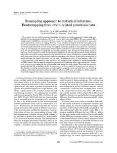
Figure­11: Simulated Scene Consisting of 4 Tanks & 3 Trucks (left), Infrared Image Y1 (middle), ® P and < Y2 , ni=1 d(θi ) (right)

A A.1

Sensor Models Model for Infrared Imagery

We adopt the probability model proposed by Snyder et al. [13]. Let Y1 ∈ Rr×c be an image (matrix) as in the right panel of Figure 11. Let q denote the locations of targets contained in the true scene. Let z be a typical pixel in the image Y1 . Then Y1 (z) = P (z) + R(z) + D(z) + B(z) where each term in the sum is a random variable: P (z) ∼ Poisson((I0 ∗ h)(z));R(z) ∼ N (µR , σ 2 R ) is readout noise at z; D(z) ∼ Bernoulli(p) accounts for a dead pixel at z; B(z) ∼ N (µB , σ 2 B ) is black current at z. The Poisson mean at z is the P convolution of the ideal image I0 with the point spread function h of the IR camera: I0 (z) = ni=1 Tαi (z − qi ), where Tαi is a 2-dimensional type-αi template of the ith target vehicle, qi is the location of the ith target vehicle, and n is the number of target vehicles in the scene. The distribution of Y1 (z) is rather complicated. For simplicity, we currently ignore the contributions of R(z), D(z), and B(z). The infrared camera can detect all aspects of the scene (g1 (X) = X) and we assume that Y1 (z1 ), . . . , Y1 (zrc ) are conditionally independent given X. These assumptions lead to a Poisson likelihood function for Y1 . In what follows, computations are performed using a Gaussian likelihood function justified via the near-field approximation: L1 (Y1 | X) =

³ 1 ´ 1 exp − 2 kY1 − I0 ∗ hk2F , Z 2σ1

(6)

where k · kF is the Frobenius norm of a matrix, σ12 is the variance of Y1 , and Z is a normalizing constant. Underlying this approximation is the assumption that the infrared camera receives a strong signal. This means that the Poisson rate parameters (I0 ∗ h)(zi ) tend to be large and we may interpret each Y1 (zi ) as a sum of independent Poisson(1) random variables. The near-field approximation follows as an application of the Central Limit Theorem.

A.2

Model for Acoustic Data

We adopt the probability model commonly used in array signal processing detailed in Miller et al. £ ¤0 [8]. Let Y2 (t) = Y21 (t), . . . , Y2m (t) be the acoustic signal at time t received by a linear array of m equally spaced sensors. For the ith of n target vehicles, let θi be the angle at which the planar sound waves wash over the sensor array. We take the θi s to be constant in t by Passuming that each target is stationary when its signal moves over the sensor array. Then Y2 (t) = ni=1 ai (t)d(θi )+w(t) where: (i) ai (t) is the amplitude of the signal from the ith target vehicle at time t; (ii) d(θi ) ∈ Cm

18

is the direction vector associated with the signal from the ith target vehicle and is given by £ ¤0 d(θi ) = 1, exp{−jπ cos(θi )}, . . . , exp{−(m − 1)jπ cos(θi )} (j 2 = −1); (iii) w(t) ∈ Cm is complex-Gaussian observation noise at time t with