1
A Model-based sequence similarity with application to handwritten word-spotting Jose A. Rodriguez-Serrano and Florent Perronnin IEEE Transactions on Pattern Analysis and Machine Intelligence, 34 (11), pp. 2108-2120, Nov. 2012.
http://ieeeexplore.com/xpl/freeabs all.jsp?reload=true&arnumber=6133288 c
2012 IEEE. Personal use of this material is permitted. Permission from IEEE must be obtained for all other uses, in any current or future media, including reprinting/republishing this material for advertising or promotional purposes, creating new collective works, for resale or redistribution to servers or lists, or reuse of any copyrighted component of this work in other works.
IEEE TRANSACTIONS ON PATTERN ANALYSIS AND MACHINE INTELLIGENCE
2
A Model-based sequence similarity with application to handwritten word-spotting Jose´ A. Rodr´ıguez-Serrano and Florent Perronnin Abstract—This article proposes a novel similarity measure between vector sequences. We work in the framework of modelbased approaches, where each sequence is first mapped to a Hidden Markov Model (HMM) and then a measure of similarity is computed between the HMMs. We propose to model sequences with semi-continuous HMMs (SC-HMMs). This is a particular type of HMM whose emission probabilities in each state are mixtures of shared Gaussians. This crucial constraint provides two major benefits. First, the a priori information contained in the common set of Gaussians leads to a more accurate estimate of the HMM parameters. Second, the computation of a similarity between two SC-HMMs can be simplified to a Dynamic Time Warping (DTW) between their mixture weight vectors, which reduces significantly the computational cost. Experiments are carried out on a handwritten word retrieval task in three different datasets - an in-house dataset of real handwritten letters, the George Washington dataset and the IFN/ENIT dataset of Arabic handwritten words. These experiments show that the proposed similarity outperforms the traditional DTW between the original sequences, and the model-based approach which uses ordinary continuous HMMs. We also show that this increase in accuracy can be traded against a significant reduction of the computational cost. Index Terms—Handwriting recognition, word spotting, image retrieval, hidden Markov model.
✦
1
I NTRODUCTION
T
Here exist many pattern recognition problems where the objects of interest can be represented with ordered sequences of vectors, also referred to as multi-dimensional time series. This includes speech recognition [1], [2], [3], biological sequence processing [4], video analysis [5], on-line handwriting recognition [6] and offline handwriting recognition [7], [8], among others. Defining good measures of similarity between vector sequences is fundamental for applications such as information retrieval, density estimation, clustering, K-nearest-neighbor or kernel classification. The application of interest in this work is handwritten word-spotting, where the goal is to detect specific keywords in handwritten document images. This problem has attracted a lot of interest from the computer vision community [9], [10], [11], [12], [13], [14]. This is a very challenging task as different occurrences of the same handwritten word may have significantly different appearances owing to different writing styles, segmentation errors, spelling mistakes, noise and other sources of variability (c.f. Figure 1). More precisely we will focus on the query-by-example (QBE) paradigm, which consists in retrieving candi• J.A. Rodr´ıguez-Serrano is with the Textual and Visual Pattern Analysis group, Xerox Research Centre Europe, Meylan, France. Parts of the work were carried out while he was with the Computer Science department at Loughborough University, and with the School of Computing at the University of Leeds. E-mail:
[email protected] • F. Perronnin is with the Textual and Visual Pattern Analysis group, Xerox Research Centre Europe, Meylan, France. E-mail:
[email protected]
Fig. 1. Different occurrences of the same handwritten word with different writing styles, segmentation errors and noise.
date word images which are similar to a given query word image. In this context, words are represented as sequences of feature vectors. Therefore, the quality of the matching directly depends on the measure of similarity between such sequences. This article proposes a model-based similarity between vector sequences with application to word-spotting. The remainder of the introduction discusses the related work in the areas of word-spotting and model-based similarity measures and describes our contribution. 1.1 1.1.1
Related Work QBE handwritten word-spotting
The QBE handwritten word-spotting paradigm can be formulated as a classical image retrieval problem. A query word image is compared with a set of candidate
IEEE TRANSACTIONS ON PATTERN ANALYSIS AND MACHINE INTELLIGENCE
3
word images in a database and the system returns the most similar images [10], [11], [15] or, more generally, ranks all candidates in descending order of similarity to the query. This is to be contrasted with the query-bytext (QBT) paradigm [16], [9], [17] where the input is the text string to be searched. This can be achieved using techniques which are very close to classical handwriting recognition [18]. QBE and QBT systems have merits of their own. On the one hand, QBT systems possess all the advantages of handwriting recognition systems, such as the flexibility to search for any keyword or the possibility to leverage large amounts of labeled data when available. On the other hand, the influential work by Manmatha et al. [10] demonstrates that a QBE approach based solely on image matching , i.e. which does not require a supervised training phase, can obtain sufficient accuracy to be useful in a practical scenario. QBE is therefore especially interesting in cases where labeled data is not available or would be costly to obtain. For this reason, a QBE system can be easily ported to a new domain (e.g. historical documents vs modern mail) or a new language (e.g. English vs Arabic) as shown in our experiments. The two important components of a QBE system are thus the representation (image descriptor) and the matching (measure of similarity between descriptors). Regarding the representation, earlier works employed holistic descriptors, i.e. the whole image is represented with a single fixed-length feature vector, as in [10] or [19]. However, in state-of-the-art approaches to handwriting recognition and word spotting it is more common to describe a word image as a sequence of feature vectors [7], [11], [8], [20]. Typically, a sliding window traverses the image from left to right and a feature vector is extracted at each position. See [21] and [20] for comparisons of sequential descriptors for the specific problem of word-spotting. As for the matching, the most common distance between two time series, also adopted in the word image retrieval literature [21], [22], [23], is DTW [24]. It consists in finding the optimal elastic alignment (warping path) between the vectors of the two sequences and then accumulating the individual vector-to-vector distances along the warping path.
sequences. In the latter case, the probabilistic model can be trained with all the sequences contained in the set. This framework has been successfully applied to image classification and retrieval where images can be described by unordered vector sets (i.e. bag-of-patches). Images can thus be described by discrete distributions, i.e. histograms (e.g. [25]), or continuous distributions, typically Gaussian mixture models (GMMs) (e.g. [26]). Although such orderless approaches have been used in the past for printed and handwritten matching [27], we found them to be insufficient for our problem as the order of vectors contains highly discriminative information. Jebara et al. [28] proposed to apply a similar framework for time series. The probability distribution for a sequence is obtained by training a continuous HMM (C-HMM). Then the probability product kernel (PPK) [29] is employed to compute a similarity between HMMs. For simple clustering tasks (one of them, interestingly, of word images) the authors report better results than other kernels and HMM-based clustering methods. One of the major issues with model-based distances is the training of the probabilistic model for a single sequence. Because the number of C-HMM parameters grows linearly with the number of states, it is important to keep the number of states as well as the number of parameters per state small (i.e. the number of Gaussians) to avoid over-fitting when considering a single sequence (or few sequences). For the simple 2-class clustering experiments reported in [29] a very small number of states (from 2 to 4) and Gaussians per state (a single one) was sufficient for good performance. This is an unrealistic setting in several applications and especially in our word image retrieval scenario. Usually, word models are left-to-right C-HMMs with several states per character (typically on the order of 10), meaning that a word is modeled with several tens of states [7], [8]. In section 5.1.2 we confirm this limitation experimentally and show that a model-based approach can actually perform worse than a standard DTW.
1.1.2 Model-based similarities. In the field of pattern recognition, model-based similarities were shown to be powerful tools to measure the similarity of vector sets. Computing these distances consists of two steps: (i) mapping each vector set to a probability distribution, and (ii) computing a similarity in the distribution space. One advantage of model-based distances is that they compress the information of the vectors sets in a reduced number of parameters. Another advantage is that they provide a principled way to compute a distance between individual vector sequences as well as between sets of
We believe that a crucial but unexploited advantage of model-based similarities for vector sequences is the possibility to incorporate a priori information in the model. The main contribution of this work 1 is to model vector sequences with a semi-continuous HMM (SC-HMM): the SC-HMM Gaussians are constrained to belong to a word-independent shared pool of Gaus-
1.2
Our Contributions
1. A preliminary conference version of the paper was presented in [30]. The present version provides a greater level of detail, additional figures, and a significantly extended experimental validation (with new experiments in two additional datasets and in a trajectory matching scenario).
IEEE TRANSACTIONS ON PATTERN ANALYSIS AND MACHINE INTELLIGENCE
sians, referred to as “universal” GMM. This provides two major benefits: 1) The shared GMM may be learned offline from a large set of descriptors. The GMM describes the visual primitives which are present in word images (letters, parts of letters, connectors between letters, etc.) and captures information about the domain of interest, i.e. about the specific language (and especially the alphabet) and the type of document which are being considered. The remaining SC-HMM parameters are estimated from the sequence itself. Mixing sequence-independent (but domain-dependent) and sequence-dependent information provides a more robust estimate of the model parameters. 2) Because all the states of the SC-HMMs share the same set of Gaussians, only the mixture weights contain sequence-specific information (the information contained in transition probabilities is disregarded). We will show that we can simplify the distance between two SC-HMMs as the DTW between two sequences of weight vectors. This results in a huge reduction of the computational cost. While our work focuses on handwriting, we underline that the proposed measure of similarity is applicable to any problem where one needs to compute a measure of similarity between sequences. Actually, in section 6.2 some experiments are carried out on a trajectory clustering task to illustrate the generality of the approach. The remainder of the paper is structured as follows. In section 2 we explain how a sequence is modeled with a SC-HMM and how the SC-HMM parameters are trained. In section 3, we consider the computation of distances between SC-HMMs. In section 4, we summarize the full similarity computation process. In section 5 we show experimentally the effectiveness of our approach on a word image retrieval task. We show that the proposed approach outperforms a DTW baseline as well as the model-based approach proposed in [28]. We also show that this increase in retrieval accuracy can be traded against a significant decrease of the retrieval speed. Finally, in section 6 conclusions are drawn and we show that the proposed similarity measure is general and can be applied beyond handwritten word-spotting. In the remainder of this text, we will use the terms similarity / dissimilarity interchangeably as one can be converted into the other in a trivial way.
2 R EPRESENTING SC-HMM
A
S EQUENCE
WITH A
The first step of the proposed method consists in estimating an HMM with a sequence of T vectors X = {x1 . . . xT } extracted from a word-image. In this section, we first describe the parametrization of our
4
SC-HMM. We then explain how to train the SC-HMM parameters. 2.1
Parametrization
HMMs [31] are generative models for sequences which assume the existence of a finite state space of N values: S = {1, . . . , N }. At each time t the system is assumed to be in a hidden state, which can be represented with a discrete latent variable qt ∈ S. Each state models the distribution of features for a piece of the sequence. An HMM is described by three types of parameters: • Initial occupancy probabilities: πi = P (q1 = i), • Transition probabilities: ai,j = P (qt = j|qt−1 = i). In the following, we will focus on a particular case of HMM commonly used in handwriting and speech recognition, the left-to-right HMM with no skip-state jump, which has the following properties: ai,j = 0 if j 6= i or j 6= i + 1, π1 = 1, πi = 0 if i > 1. • Emission probabilities: p(xt |qt = i). In the case of continuous observations, the emission probabilities are generally assumed to be GMMs. We will assume diagonal covariance matrices since their computational cost is reduced and any distribution can be approximated with arbitrary precision by a mixture of Gaussians with diagonal covariances. The number of states N of the model is chosen as a factor ν (with 0 < ν ≤ 1) times the length T of the sequence : N = νT . The parameter ν will later be referred to as “compression” factor because intuitively the HMM compresses in νT states the information contained in T observations. To model sequences, we propose to use a particular type of HMM, namely the SC-HMM [32]: the emission probabilities of all states in all SC-HMMs share the same set of K Gaussian components. Let pk denote the k-th Gaussian with mean vector µk and standard X deviation vector σk . Let us call wik the mixture weight for the Gaussian k at state i of the SC-HMM trained from X. The emission probability in state i of the SCHMM trained from X is given by: p(xt |qt = i) =
K X
X wik pk (xt ).
(1)
k=1
The intuition behind the SC-HMM is that different sequences can be adequately described by the same set of visual primitives (characters, parts of characters, connectors between characters, etc.) each local primitive being modeled by a different Gaussian. What characterizes the state of a given sequence (and therefore the corresponding part of the sequence) is the set of Gaussians which are “picked”. The crucial point in this paper is that we can learn the parameters µk and σk offline from a large separate unlabeled
IEEE TRANSACTIONS ON PATTERN ANALYSIS AND MACHINE INTELLIGENCE
5
sample set of sequences and then use X to estimate X the remaining parameters aX i,j and wi,k . Therefore, we refer to µk and σk as sequence-independent (i.e. shared) X parameters and aX i,j and wi,k as sequence-dependent parameters. This separation provides a major advantage: the shared Gaussians inject prior domain information and prevent overfitting. We now briefly describe the two separate steps of the SC-HMM training: (i) the training of the sequenceindependent GMM parameters (ii) the training of the sequence-dependent parameters. 2.2 Sequence-independent parameters Since the shared Gaussians are supposed to describe the distribution of descriptors in any sequence, we propose to train a GMM from a large set of descriptors using Maximum Likelihood Estimation (MLE) and to inject its Gaussians in the SC-HMM models. The mixture weights of this GMM are discarded and replaced by the learned sequence-dependent mixture weights (c.f. next subsection). To train the GMM, the order of the feature vectors extracted from a sequence is disregarded. In our word-image retrieval problem, the training material should consist of a large set of descriptors extracted from a wide variety of images corresponding to different words and (when applicable) different writing styles. The learned GMM is referred to as domain-GMM since it encodes domain-specific information. For instance, we expect the learned GMMs to be very different in the cases where they are learned from a dataset of French words or Arabic words or when they are learned on modern mail or historical documents. The algorithm of choice for MLE is ExpectationMaximization (EM) [33]. To train a GMM, we employ the iterative strategy implemented in HTK [34] which was inspired by the Linde-Buzo-Gray (LBG) vector quantization algorithm [35]. We start from a single Gaussian for which there exists a closed form formula. Given a GMM with K Gaussians, we obtain a GMM with 2K Gaussians by splitting each Gaussian into two. More formally, each Gaussian parametrized by (wk , µk , σk ) is split into two Gaussians parametrized respectively by (wk /2, µk + ǫσk , σk ) and (wk /2, µk − ǫσk , σk ). ǫ is a small perturbation parameter, e.g. set to ǫ = 0.01. After this splitting step, the usual EM re-estimation algorithm is run. The splitting and EM-retraining process is repeated until the desired number of Gaussians is obtained. This process enables to monitor the model accuracy as a function of its complexity (i.e. the number of Gaussians). To illustrate the visual vocabulary obtained, we analyze the case of the features proposed by Vinciarelli et al. [8]. Here, a sliding window of width w pixels is split into a 4x4 grid, and the number of black pixels inside each cell is counted (assuming binary images). We select this example since it allows an easy visual
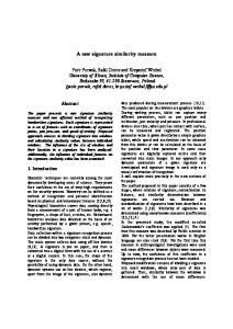
Fig. 2. Means of the Gaussians (visual vocabulary) obtained for the Vinciarelli et al. features in the case of 64 Gaussians. The GMM was estimated on a separate set of L = 106 feature vectors extracted from many different word images. The number on top of each visual word displays its relative importance as measured by wi L.
interpretation: each feature vector can be displayed as a 4x4 image where the intensity of the cell is proportional to its value. Fig. 2 displays the means of the obtained Gaussians when estimating a domainGMM with 64 components on a set of descriptors extracted from word images in French letters. 2.3
Sequence-dependent parameters
Once the parameters µk and σk , k = 1 . . . K have been trained offline, the remaining parameters aX i,j X and wi,k can be learned from a particular sequence X. Again, we use the MLE criterion and the estimation is performed iteratively via the EM algorithm. Let γi (t) = p(qt = i|X) be the probability that xt was generated by state i. We denote by mk (t) the discrete latent variable indicating which mixture component (i.e. Gaussian) emitted xt . Let γik (t) = p(qt = i, mt = k|X) be the probability that xt was generated by state i and mixture component k. Finally, let ξij (t) = p(qt = i, qt+1 = j|X) be the probability that xt was generated by state i and xt+1 by state j. During the E-step, the posteriors γi (t), γik (t) and ξij (t) are computed based on the current estimate of parameters using the forward-backward algorithm (e.g. see [31]). During the M-step, the parameters are re-estimated: PT −1 ξij (t) , a ˆi,j = Pt=1 T −1 t=1 γi (t) PT γik (t) w ˆi,k = PT t=1 . PN t=1 n=1 γin (t)
(2) (3)
IEEE TRANSACTIONS ON PATTERN ANALYSIS AND MACHINE INTELLIGENCE
The sequence-dependent parameters are initialized with a “flat start” strategy, which divides the training into two rounds of EM iterations. In the first round, the sequence X is split regularly into N states and a few EM iterations are run to estimate the state parameters without letting the state variable change. This is a common procedure to initialize left-to-right models. After that we set the transition probabilities to ai,i = ai,i+1 = 0.5 and ai,j = 0 for j 6= i, i + 1, ∀i, j = 1 . . . N . Then, the state restriction is removed and the usual EM iterations are applied. We note that in the limit case where the number of states is N = 1, then all the order information is lost and the sequence X is simply characterized by the number of soft occurrences of each of the visual primitives, i.e. by a soft bag-of-visual words [25]. Hence, the SC-HMM can be viewed as an extension of the soft bag-of-visual-words to sequences.
3 A M EASURE SC-HMM S
OF
6
in considering the possible alignments between the state sequences of two HMMs. The main difference between these methods is in the choice of the local measure of similarity between states: Bayes probability of error [6], Kullback-Leibler (KL) divergence [3], [2] or Bhattacharyya similarity [36], [28]. Another difference is whether one considers the best path [6], [2] or a sum over all paths [36], [3], [28]. We follow [6], [2] and consider only the best path. As suggested in [2], we also disregard the transition probabilities as they seem to contain little discriminant information in the case of left-to-right topologies (as is the case in handwriting and speech recognition). Under these two approximations, the distance computation between two HMMs simplifies to a DTW between state sequences. In the following, we briefly review the DTW algorithm and then explain how to exploit it to define a distance between states (i.e. between GMMs).
S IMILARITY B ETWEEN
Computing a measure of similarity between two sequences is now tantamount to computing a measure of similarity between two SC-HMMs. In this section, we first briefly review existing measures of similarity between HMMs (especially C-HMMs). We then specialize the measure to our SC-HMM case. 3.1 Measures of similarity between C-HMMs There is an abundant literature on the computation of similarities / dissimilarities between C-HMMs. In [6] Bahlmann and Burkhardt propose a method for comparing HMMs based on the Bayes probability of error (the area of overlap between two probability density functions) with the goal of analyzing letter misclassification for an online handwriting recognition system. In [1], Singh et al. are interested in measuring the distance between sound units to improve a speech recognition system. The distance between two HMMs is computed using the Kullback-Leibler (KL) divergence. Since there is no closed-form formula for the KL divergence between two HMMs, it is approximated using Monte Carlo sampling. In [2], Huo and Li propose to represent a word as a sequence of state-dependent GMMs and measure the distance using a DTW between sequences of GMMs. The Kullback-Leibler (KL) divergence is used to compute the distance between two GMMs (see also [2] for many references on distances between HMMs). In [28] Jebara et al. propose an algorithm reminiscent of forward-backward for the computation of the PPK between two C-HMMs. In [3] and [36], Hershey and his colleagues derive variational bounds between CHMMs for the KL divergence and Bhattacharyya similarities respectively. In the case of left-to-right HMMs all these algorithms boil-down to the same principle: they consist
3.2
Dynamic time warping
DTW is an elastic distance between vector sequences. Let us consider two sequences of vectors X and Y of length TX and TY respectively. DTW considers all possible alignments between the sequences, where an alignment is a set of correspondences between vectors such that certain conditions are satisfied. For each alignment, we determine the sum of the vector-tovector distances and define the DTW distance as the minimum of these distances or, in other words, the distance along the best alignment, also referred to as warping path. The direct evaluation of all possible alignments is prohibitively expensive, and in practice a dynamic programming algorithm is used to compute a distance in quadratic time. It takes into account that the partial distance DTW(m, n) (where m = 1 . . . TX and n = 1 . . . TY ) between the subsequences {x1 . . . xm } and {y1 . . . yn } can be determined as DTW(m − 1, n) DTW(m − 1, n − 1) +d(m, n), DTW(m, n) = min DTW(m, n − 1) (4) where d(m, n) is the vector-to-vector distance between xm and yn , referred to as local distance - usually the Euclidean distance. In practice, dividing the DTW distance by the length of the warping path leads to an increase in performance. The local distance d(., .) may be replaced by a local similarity. This simply requires changing the min into a max in Eq. (4). Because one can apply Eq. 4 to fill the matrix DTW(m,n) in a row-by-row manner, the cost of the algorithm is in O(TX TY D) where D is the dimensionality of the feature vectors. To extend DTW to state sequences, it is sufficient to replace the local vector-to-vector distance d(., .) by
IEEE TRANSACTIONS ON PATTERN ANALYSIS AND MACHINE INTELLIGENCE
a local state-to-state distance. This is the object of the next section.
where IN is the N × N identity matrix, and thus the distance between two states simplifies to M X
3.3 Distances between states We now have to address the problem of defining a distance between states, i.e. between GMMs. In the case of SC-HMMs, the only sequence-dependent state parameters are the mixture weights. Hence, the distance between two states may be defined as the distance between two vectors of mixture weights. In this work we focus on the PPK as a measure of similarity between GMMs for a fair comparison with [28] but other measures such that the KL divergence could have been employed. We will now show that in the case of the Bhattacharyya similarity this can be related to the true Bhattacharyya similarity between the GMMs. In the PM PN following, f = i=1 αi fi and g = j=1 βj gj denote two GMMs (fi and gj are the Gaussians and αi and βj the mixture weights). We denote by α = [α1 . . . αM ]T and β = [β1 . . . βN ]T the two weight column vectors. The Probability Product Kernel (PPK) [29] is defined as: Z ρ ρ (f (x)g(x)) dx. (5) Kppk (f, g) = x
The Bhattacharyya similarity corresponds to the spe1/2 cial case B(f, g) = Kppk (f, g). There is no closedform formula for B in the case where f and g are GMMs and we have to resort to approximations. We can however use the following upper-bound: B(f, g) ≤
M X N X
(αi βj )1/2 B(fi , gj )
(6)
i=1
where the square-root denotes a term-by-term operation. We note however that the computational cost remains quadratic in the number of Gaussians (typically, from a few tens to a few hundreds). This cost might be too large for most applications of practical value. Therefore, we do the following additional approximation on the bound. We assume that the Gaussians are well-separated, i.e. B(fi , fj ) ≪ B(fi , fi ) for j 6= i. Empirically, we observed that this approximation is all the more likely to be good as the dimensionality of the feature space increases. As we have by definition B(fi , fi ) = 1, this leads to the approximation B ≈ IN ,
(αi βi )1/2 =
√ Tp α β
(8)
which is the discrete Bhattacharyya distance between the weight vectors α and β. If one stores the square roots of the weight vectors, this quantity is extremely efficient to compute (dot product).
4
S UMMARY
For completeness, we provide a summary of the steps required to compute the proposed similarity measure between two sequences X and Y of length TX and TY respectively. Fig. 3 illustrates the process graphically. 1) Train offline a domain-GMM with K Gaussians pk from a large number of samples (c.f. section 2.2). Inject these Gaussians in the SC-HMM emission probabilities. 2) Estimate the mixture weights and transition probabilities of the SC-HMM using X as unique training sample. We call NX = νTx the number of states of this HMM. We do the same for Y . X 3) We recall that wik denotes the mixture weight for the Gaussian k at state i of the SC-HMM obtained from X. Let us use the vector notation X X wiX = [wi1 . . . wiK ] to express compactly all the weights of state i. Since in a left-to-right HMM the states are ordered, the weights of the SCHMMs can be viewed as a sequence of vectors. Let WX and WY be respectively the sequences of vector weights for sequences X and Y :
i=1 j=1
The values B(fi , gj ) correspond to the Bhattacharyya similarities between pairs of Gaussians for which a closed form formula exists (see for instance [29]). In the case of SC-HMMs, we recall that the GMM emission probabilities are defined over the same set of Gaussians, i.e. M = N , fi = gi and the values bi,j = B(fi , fj ) may be pre-computed. Let us denote by B the N × N matrix with entries bi,j . In such a case, the similarity between two states is just: √ T p α B β (7)
7
X } WX = {w1X . . . wN X Y } WY = {w1Y . . . wN Y
(9)
The distance between X and Y is defined as the DTW between WX and WY . If K is the number of Gaussians in the shared pool, then the cost of the DTW between WX and WY is in O(ν 2 TX TY K). In our experiments, we used the Bhattacharyya similarity (Eq. 8) as local measure of similarity for the DTW. Hence, the only parameters to tune in our distance measure are the value of the compression factor ν and the number of Gaussians K.
5
E XPERIMENTS ON HANDWRITTEN WORD IMAGE RETRIEVAL The proposed similarity measure is evaluated in the context of a handwritten word image retrieval task. The problem consists in querying a dataset of handwritten documents with a query word image and in returning word images that belong to the same word class. This task is very popular in the domain of digital libraries, where documents can be represented
IEEE TRANSACTIONS ON PATTERN ANALYSIS AND MACHINE INTELLIGENCE
8
Fig. 3. Diagram summarizing the proposed similarity between vector sequences
as sets of word images [10]. Because obtaining a transcription is costly and OCR systems for handwritten text do not yet show satisfying accuracy, word image retrieval can be used to enable searches or indexing, among others. Classically, word image retrieval has been formulated as a problem of image matching. Images are represented using sequences of feature vectors and the common distance measure between word images has been DTW. In this evaluation, we use the proposed similarity measure for image matching purposes. We compare it to a classical DTW and to the PPK of Jebara et al. [28]. First, a detailed evaluation is conducted on a large in-house dataset with more than 180K word images. Then, results are validated on two other public datasets: the George Washington dataset, common in the word spotting community and popularized in [10],[11], and the IFN/ENIT database of handwritten Arabic words [37]. 5.1 French handwritten letters dataset 5.1.1 Experimental setup Dataset: The French letters dataset is an in-house dataset employed in the context of an industrial wordspotting application. It consists of 630 scanned handwritten letters (in French) mailed to the customer department of a corporation. Therefore, this is real data and as such is challenging for a retrieval task because of the variety of writing styles and other difficulties such as spontaneous writing, spelling mistakes, noise, etc. Fig. 4 shows examples of such letters. The dataset is split into three parts: D1 (105 documents) is used to estimate the GMM, D2 (420 documents) is used for validation, and D3 (105 documents) is used as test set to show how our measure can extrapolate to new queries. Pre-processing: A segmentation process extracts word image hypotheses from the documents. This
Fig. 4. Samples from the French letter dataset. Black frames were only used to hide sensitive information for the purpose of display in this article and did not appear in the original dataset.
generates approximately 150K word hypotheses for D2 and 30K for D3. The word images are normalized with respect to skew, slant and size as in [7]. Labeling: A subset of word hypotheses is labeled with 10 word identities which are relevant to the type of documents considered (e.g. “contrat”, “abonnement”, “r´esilier” which can be translated as contract, subscription and cancel, respectively). The number of sample per class varies from 170 to 625 in D2. These numbers should be compared to the 150K segmented word-hypotheses: the probability that these samples appear by chance among the top retrieved results is very small. Feature extraction: Features are then obtained for all the images by sliding a window from left to right and computing for each window a set of features. To assess the generality of the proposed approach, the evaluation is carried out on three state-of-the-art feature types, namely: (i) the column features by Marti and Bunke [7], (ii) the zoning features by Vinciarelli et al. [8] and (iii) the LGH features by Rodr´ıguez and
IEEE TRANSACTIONS ON PATTERN ANALYSIS AND MACHINE INTELLIGENCE
Perronnin [20] which are very similar to the SIFT descriptors used for object detection [38]. Pruning: A fast, word classifier based on holistic features is previously trained on keyword images and is used to score the candidate images prior to the distance computation. Setting a conservative threshold allows to quickly reject many unlikely matches so that the distance computation focuses only on a reduced set of similar samples. Details about this pruning strategy are given in [39]. Validation / test: Experiments are organized in two runs: (i) a validation run which assesses the behavior of the system for different parameters, and (ii) a test run where the competing systems are compared with their best performing parameters (as measured on the validation run) on a set of novel queries. For the validation experiments, D2 is split into 4 folds. 10 samples from each word class are selected randomly from each fold and used to query against the remaining folds. This guarantees that the queried and retrieved images are from different writers. For each of the 400 queries (10 samples × 4 folds × 10 classes) the retrieval performance is evaluated using average precision (AP). Overall results are reported by computing the mean over all the runs (mean AP or shortly mAP). For the test experiments, 10 samples from each word class are selected from D3 and queried against D2. Comparison: The proposed similarity measure is compared to DTW and PPK between C-HMMs: • For DTW we adopt the most common option in the word retrieval literature [11] of using the Euclidean distance as a local distance, and then dividing the final distance by the length of the warping path. We also implemented a SakoeChiba band to keep the solution (i.e. the optimal path) within a reasonable distance of the diagonal and therefore to avoid unreasonable stretch effects. • In PPK experiments, the number of states is chosen as a constant times the width of the word (as is the case of our method). We tuned this value on the validation set to optimize the performance. In validation experiments, it was found that the best factor for the Marti and Bunke and Vinciarelli features was 0.2 while it was 0.05 for the LGH features. This confirms the fact that a small number of states is required to avoid over-fitting, as stated in the introduction. Following [28], we choose ρ = 1/2, i.e. the similarity between two states is measured using the Bhattacharyya kernel. This choice makes sense since it leads to a normalized measure: the similarity between two states (and therefore between two C-HMMs) is maximal if and only if the two states (and therefore the two C-HMMs) are equal. Note that this would not be necessarily the case for other choices of ρ. The C-
9
•
HMMs were trained with a single Gaussian per mixture as this led to the best performance and is consistent with the setting of [28]. For the proposed distance, we also choose ρ = 1/2 to measure the similarity between two weight vectors. The primary motivation behind this choice is to enable a fair comparison with PPK. Indeed, we showed in section 3.3 that the Bhattacharyya kernel between two GMMs with the same Gaussians could be approximated by the Bhattacharyya kernel between their weight vectors. Hence we use similar measures between states for PPK and the proposed distance which enables to focus on the merits of these two frameworks, not of the underlying metrics.
5.1.2 Parameter influence We now evaluate the influence of the two main parameters of our measure: the number of Gaussians and the compression factor. Number of Gaussians. For this first set of experiments, we choose as compression factor for the proposed algorithm the value ν = 1 (i.e. no compression). In this degenerate case, we train an HMM with T states with a sequence of T vectors. This shows how much our similarity measure is resilient to overfitting. Fig. 5 shows the mAP (in %) on the validation set for the Marti and Bunke features, Vinciarelli features and LGH features respectively as a function of the number of Gaussians. We can observe on the three figures that the proposed similarity outperforms DTW and PPK even for a fairly small number of Gaussians. Compression factor. In applications where efficiency is important, one might accept to trade retrieval accuracy against speed. We recall that the cost of the original DTW is in O(TX TY D) (c.f. section 3.2) while the cost of the proposed algorithm is in O(ν 2 TX TY K) 2 (c.f. section 4), with 0 ≤ ν ≤ 1. Let us analyze the behavior of the proposed measure with respect to the value of the compression factor. Fig. 6 shows the validation performance of the proposed method compared to the DTW performance line, for a varying length factor, for the three types of features. We chose a number of Gaussians K as close as possible to the dimensionality of the features D: K = 8 and D = 9 for the Marti and Bunke features, K = D = 16 for the Vinciarelli features and K = D = 128 for the LGH features. If K = D, then a compression factor ν leads to a reduction of the computational cost by a factor O(1/ν 2 ). In all three figures we basically observe a decrease in performance as ν goes down. This suggests a 2. Note that the metric between two descriptors used by DTW is the Euclidean distance while the metric between two weight vectors for the proposed measure is the dot product (assuming that the weight vectors have been pre-square-rooted). The cost of computing efficiently a Euclidean distance and a dot-product are very similar (and even equivalent in the case where the descriptors are L2 normalized).
IEEE TRANSACTIONS ON PATTERN ANALYSIS AND MACHINE INTELLIGENCE
10
0.25 0.2
mAP
mAP
0.1 0.15 0.1 0.05 Proposed DTW PPK
0.05 0 2
4
Proposed DTW 0
8 16 32 64 128 256 512 Number of Gaussians
0.1 0.2
0.4
ν
0.6
0.8
1
0.25 0.15
0.15
mAP
mAP
0.2
0.1
0.1 0.05 Proposed DTW PPK
0.05 0 2
4
Proposed DTW 0
8 16 32 64 128 256 512 Number of Gaussians
0.3
0.1 0.2
0.4
ν
0.6
0.8
1
0.3
0.25 0.2 mAP
mAP
0.2 0.15
0.1
0.1 Proposed DTW PPK
0.05 0 2
4
8 16 32 64 128 256 512 Number of Gaussians
Fig. 5. Comparison of the proposed measure of similarity with DTW and PPK. We study the influence of the number of Gaussians in the SC-HMM on the retrieval accuracy. From top to bottom: Marti & Bunke, Vinciarelli and LGH features.
Proposed DTW 0
0.1 0.2
0.4
ν
0.6
0.8
1
Fig. 6. Influence of the compression factor ν on the retrieval accuracy. From top to bottom: Marti & Bunke, Vinciarelli and LGH features.
TABLE 1 mAP values on the test set for the French letter dataset
simple way of tuning this parameter: higher values for improved accuracy and smaller values for improved speed. Quantitatively, for the best features (the LGH features), even for ν = 0.1 our method performs on par with DTW. This corresponds to a reduction of the computational cost on the order of 100. In the case of the less robust features, the reduction is not quite as impressive but still significant: on the order of a factor 3 for the Bunke features (ν = 0.6) and a factor 6 for the Vinciarelli features (ν = 0.4). Note that this does not take into account the time that our algorithm takes to train the sequencedependent parameters of the SC-HMMs. However, in a retrieval scenario, word models would generally be precomputed.
set results are shown in Table 1 and it is clear that the proposed system outperforms both DTW and PPK. It is important to note that the sophisticated PPK performs significantly worse than the simple DTW baseline. These results prove that using a priori information can greatly reduce over-fitting and significantly improve the retrieval accuracy.
5.1.3 Test set results Here, each system was evaluated using the best parameters obtained in the validation experiments. Test
In the remainder of the experiments the PPK is discarded due to its inferior performance and comparisons will be carried out against DTW only (the best of the two baselines).
Method PPK DTW Proposed
Marti and Bunke 0.134 0.194 0.248
Vinciarelli 0.120 0.202 0.251
LGH 0.207 0.298 0.323
IEEE TRANSACTIONS ON PATTERN ANALYSIS AND MACHINE INTELLIGENCE
11
TABLE 2 Comparison of retrieval performances in the George Washington dataset (also displaying figures for the standard deviation (std), minimum (min), and maximum (max) over the 20 test runs. Method DTW Proposed
Fig. 7. Samples of the George Washington dataset
5.2 George Washington dataset In the previous section, the proposed similarity measure has been validated in terms of accuracy and computational cost on a large in-house database. For completeness, we replicate the experiments on two public datasets in the present and the next section. 5.2.1 Experimental conditions Dataset: The George Washington dataset is a collection of historical documents written by George Washington and his assistants. Rath and Manmatha segmented 20 pages of this collection, obtaining a set of 2,381 word images [11]. Fig. 7 shows a selection of samples of this dataset. The ground-truth consists of a matrix Rij indicating whether word images i and j are relevant, i.e. of the same class. Pre-processing and feature extraction: Features extracted from segmented and normalized images are already available in the dataset. See [11] for details. Each word image is described as a sequence of 4D feature vectors (upper, lower, mean and black/white transition profiles). To make the comparison with previous works easier, we use these features although we obtained better results with more state-of-the-art features such as LGH. Rath and Manmatha [11] apply a preliminary pruning step prior to each pairwise distance computation that we also adopt. The pruning is based on width and aspect ratio. Let us assume li and lj are the respective widths of images i and j. Let 0 ≤ f ≤ 1 define a pruning factor. If 1 li li or > f, > f lj lj
(10)
then the distance between samples i and j is set to ∞. This allows discarding unlikely matches, which leads to a considerable speed-up, at the expense of wrongly discarding pairs. Retrieval: This dataset is significantly smaller than the other datasets used in this section and splitting it into a database, validation, and test set would
mAP 0.500 0.531
std 0.034 0.042
min 0.455 0.461
max 0.558 0.609
yield small subsets. Previous works (see e.g. [11]) has discounted this fact by validating and testing on the whole set. However, we adopt the more correct cross-validation procedure. The dataset is split uniformly into 5 folds. In each run we take 3 folds as the database, one fold for validating parameters and the remaining fold for testing, and repeat for all 20 different combinations of this setup. For each run we report the AP of the test set, using the best parameters obtained in the validation set. The cross-validated parameters are the pruning factor f and the number of Gaussians. We then report the mAP of the 20 runs. 5.2.2 Retrieval results Table 2 shows compares the mAPs of DTW and the proposed similarity in the George Washington dataset, for ν = 1. An improvement is observed over DTW with the proposed similarity measure. We observe that the retrieval task in this dataset is easier: for DTW we obtain mAP ≈ 50%, while for the French letters dataset we reported mAP ≈ 12%. One reason that may account for this difference is the complexity of the data. Indeed, the George Washington letters were produced by few writers with a very consistent writing style. This is to be contrasted with the French letters dataset, where data comes from more than 600 different writers. 5.3
IFN/ENIT Arabic dataset
We also run word image retrieval experiments in the IFN/ENIT dataset of Arabic handwritten words, because: (i) it contains a reasonably high number of samples compared to the George Washington dataset, (ii) the images consist of village names, and matching village name images could be useful, for instance in postal applications and (iii) it allows verifying that the proposed method is not only applicable to Roman script, but valid in other scripts, too. To the best of the authors’ knowledge, this is the first time that word spotting experiments are reported on the IFN/ENIT database. 5.3.1 Experimental conditions Dataset: IFN/ENIT [37] is a public dataset of Arabic handwritten word images. The dataset consists of 5 sets (a to e), each with approximately 6,700 word images of Tunisian town names produced by multiple
IEEE TRANSACTIONS ON PATTERN ANALYSIS AND MACHINE INTELLIGENCE
12
0.5 0.4 0.4
mAP
mAP
0.3 0.3 0.2
0.2
0.1
0.1
Proposed DTW
Proposed DTW 0 2
Fig. 8. The 10 queries selected for the ZIP code 1000
writers, together with the corresponding ground-truth annotations. We use the following protocol: a set of query images is selected from set a to be searched in set b (6,710 images). The universal GMM is estimated on set e. With regards to the query selection, the 50 most popular labels in set b are identified and 10 images of each are randomly selected from set a. Thus the total number of query images is 500. In set b, each of the selected labels has a number of occurrences ranging from 27 to 107. In Fig. 8 the ten selected samples for the city name with ZIP code 1000 are displayed. Pre-processing: In this case the images do not need to be normalized since the IFN/ENIT dataset already provides normalized images. Pruning: The same pruning strategy as in the George Washington dataset is applied here. Feature extraction: LGH features are extracted using the same parameters as for the case of the French letter dataset. Retrieval: As in the case of the French letter dataset, the AP is computed for each of the 500 query experiments and averaged to obtain a mAP value. From the 500 queries, 250 are randomly selected for validation experiments and the remaining 250 for testing experiments. As in the case of the French letter dataset, validation experiments are run with different parameter combinations and then a test run is performed with the best parameters. 5.3.2 Results Fig. 9 shows the mAP values on the validation set when varying respectively the number of Gaussians and the compression factor of the proposed similarity measure. We also show the DTW baseline. In Fig. 9 (left), the compression factor was set to ν = 1. The result is again satisfactory: the proposed similarity measure outperforms DTW for a sufficiently high number of Gaussians (64 in this case). In Fig. 9 (right), as was the case in the previous section, the number of Gaussians is set to 128 so that the weight vector sequences have the same dimensionality as the original LGH sequences. By examining this plot, it can be appreciated that at ν = 0.4 the mAP values of DTW and the proposed similarity measure are similar. However, the transformed sequences are 1/ν = 2.5
4
8 16 32 64 Number of Gaussians
128
256
0 0
0.2
0.4
ν
0.6
0.8
1
Fig. 9. Comparison of DTW and the proposed similarity measure for the IFN/ENIT dataset as a function of the number of Gaussians (left) and of the compression parameter (right).
Fig. 10. Top 25 ranked samples after a query with the top left image of Fig. 8. Images with the same label as the query are surrounded by a thick, green rectangle. Images with a different label are surrounded by a thin, red rectangle.
times shorter, making the overall comparison on the order of 6 times faster with the proposed method. Test set results are mAP=0.347 for DTW and mAP=0.416 for the proposed similarity using the best validation parameters. This represents a significant increase in accuracy. Qualitative results of the retrieval are found in Fig. 10. Here, the top 25 results after querying the system with the top left image of Fig. 8 are shown.
6 6.1
C ONCLUSIONS
AND PERSPECTIVES
Summary
This article proposes a model-based measure of similarity between vector sequences. Each sequence is mapped to a SC-HMM and a similarity between the SC-HMMs is computed. The crucial property of the SC-HMM is that the Gaussian components of the emission probabilities are shared and can be trained separately on an unlabeled set of samples. This allows injecting prior information about the specific domain into the model. For instance, in the case of unconstrained handwritten word-spotting one may want to estimate this GMM with many different word samples from many different writers. However, if one knows that the samples come from a specific writer or from degraded documents, the samples may be chosen accordingly to capture this prior knowledge about the dataset. Thanks to this property, the proposed simi-
IEEE TRANSACTIONS ON PATTERN ANALYSIS AND MACHINE INTELLIGENCE
larity is more robust than the standard DTW and also than the model-based PPK as originally proposed. The robustness of the similarity measure has been demonstrated across different domains inside the area of handwritten word image retrieval (word-spotting), namely for modern French documents, ancient English documents and Arabic documents. As commented earlier, the only action required when porting a system to a different type of data is to estimate a new domain GMM (from an unlabeled dataset), thus coming at a relatively low cost. It has also been shown than the system can compromise performance versus speed by tuning the compression parameter ν between 0 and 1, and that by going down to the same performance as DTW one can significantly speed-up the retrieval. 6.2 Beyond handwritten words As shown in the last section, the similarity measure proposed in this article has been developed in the context of handwritten images and therefore evaluated in detail in a number of handwritten image retrieval experiments. However, the proposed method is a generic similarity measure between sequences and it does not make any assumption specific to handwritten image data. We believe it is therefore beneficial to conclude this article with an illustrative experiment that demonstrates that the proposed similarity is applicable beyond handwritten image retrieval. In particular, the proposed method will be illustrated for the application of matching and clustering object trajectories. Matching trajectories of tracked objects is a fundamental problem in the field of video analysis with applications such as retrieval of trajectories for similar behavior identification [40], or clustering the trajectories to identify the typical modes of motion ([41],[42],[43]) - and possibly detecting abnormal behaviors [44]. A trajectory is nothing more than a sequence of coordinates (usually the 2D coordinates of the object motion in the ground plane). The goal of this section is to confirm experimentally that the proposed measure of similarity can also be applied to this type of data. We perform experiments on the public NGSIM database [45]3 . One of the available datasets contains millions of trajectories corresponding to vehicles tracked in a 1 km long segment of a highway. Fig. 11 illustrates a subset of 300 trajectories, randomly sampled from the dataset. It can be appreciated that there are 7 “typical” trajectory types: 5 corresponding to vehicles driving in a straight line in one of the 5 main lanes, an additional trajectory type corresponding to vehicles driving from an “on-ramp” to the highway, and finally another mode corresponding to vehicles exiting the highway 3. available at http://ngsim.camsys.com
13
3000
2500
2000
1500
1000
500
0 0
20
40
60
80
100
120
Fig. 11. Subset of trajectories from the NGSIM dataset TABLE 3 mAP values for the trajectory matching experiment Method
mAP
DTW
0.874
PPK
0.670
Proposed
0.912
via an “off-ramp”. Of course, some vehicles exhibit trajectories which do not necessarily fit into one of these modes, such as vehicles switching lanes frequently. We first perform a trajectory matching experiment. We associate a label to each of the 2,000 trajectories, denoting which of the previous trajectory types (17) the vehicle exhibits, based on the lane information available in the dataset. If a vehicle does not fit any of the existing trajectory types, it is assigned a class “0”. We use a separate subset of 2,000 trajectories for validation purposes. We compute the similarities between all possible trajectory pairs. Each score is associated a label of “1” if trajectories have the same non-zero label, and “0” otherwise. From these labeled similarity data we can compute the AP as an indicator of the matching quality. We compare the proposed measure of similarity (with the described modifications) to the direct DTW and the PPK between HMMs. In this 2D case we use full covariance matrices for PPK and the proposed method since it enables to model the correlation between the x and y coordinates, which is very important in this application. In the case of 2 dimensions, this induces a limited additional cost. Table 3 shows the AP of the compared methods with their best parameters. Again, the proposed similarity outperforms both DTW and PPK and the results exhibit a very similar behaviour to the previous experiments on document images. Finally, we illustrate the proposed similarity measure in the context of a clustering algorithm. The pairwise distance matrix computed for the previous
IEEE TRANSACTIONS ON PATTERN ANALYSIS AND MACHINE INTELLIGENCE
3000 Cluster 1 Cluster 2 Cluster 3 Cluster 4 Cluster 5 Cluster 6 Cluster 7
2500
2000
1500
1000
500
0 0
20
40
60
80
100
120
Fig. 12. Trajectory clustering results in a portion of the NGSIM dataset (best viewed in color)
3000
2500
2000
1500
1000
500
0
0
10
20
30
40
50
60
70
80
90
100
Fig. 13. Cluster medoids (representative trajectories).
experiment can be used as input to a clustering algorithm. We re-implement the self-tuning spectral clustering algorithm by Sanguinetti et al. [46] since it provides an automatic selection of the number of clusters. Figure 11 illustrates the clustering result applied to the subset of 300 images shown in Fig. 11, with each trajectory type depicted with a different color. The method correctly identifies the 7 main modes of motion. There are also many trajectories which do not belong to one particular mode of motion but they are assigned the closest mode. In order to demonstrate that the method captures the main modes of motion despite the big number of “outlier” trajectories, Fig. 13 displays the medoids of each cluster, i.e. the trajectory which has the smallest sum of distances to all the other trajectories within the same cluster. Note that the medoids clearly correspond to the 7 main modes of motion. 6.3 Perspectives The previous section has shown that the proposed similarity is applicable beyond handwritten data. We believe that other problems could also benefit from it. A clear example is signature recognition. In order to identify a person from its signature, usually an enrollment phase is required where the subject provides a few examples of the signature. Thus very small training sets are available which probably prevent the use
14
of model-based recognition such as [47]. The proposed similarity measure could be used in this case because of its properties with respect to overfitting. Also, all the signatures in the training set would be compressed into a single model and only one computation would give a similarity between the test sample and the training samples. This is to be contrasted with nearest neighbor methods [48] which would typically require as many computations as training samples. Another aspect worth investigating is the measure which is employed to compute the similarity between two weight vectors. As mentioned in section 3.3, the primary motivation for using the Bhattacharyya kernel was to offer a fair comparison with [28]. However, other measures between histograms, such as the chi2 or the intersection kernels, could have been employed. In preliminary experiments, we even found-out that tuning the ρ parameter in Eq 5 could lead to a substantial increase in accuracy. Finally, while we showed that the proposed similarity measure is robust, as it stands it is not easily indexable. The challenge now is how to make it compatible with efficient indexing schemes such as LSH. An interesting perspective is offered by kernelized LSH (kLSH) [49], where the classical LSH is generalized to any Mercer kernel. Since the proposed similarity is not a Mercer kernel, it may be worth investigating if kLSH can be adapted to that case.
R EFERENCES [1] [2] [3] [4] [5] [6] [7] [8] [9] [10] [11] [12] [13] [14]
R. Singh, B. Raj, and R. Stern, “Structured redefinition of sound units by merging and splitting for improved speech recognition,” in ICSLP, 2000. Q. Huo and W. Li, “A DTW-based dissimilarity measure for left-to-right hidden markov models and its application to word confusability analysis,” in ICSLP, 2006. J. Hershey, P. Olsen, and S. Rennie, “Variational KullbackLeibler divergence for hidden Markov models,” in ASRU Workshop, 2007. J. K. Kim and S. Choi, “Clustering sequence sets for motif discovery,” in NIPS, 2009. M. Brand and V. Kettnaker, “Discovery and segmentation of activities in video,” IEEE Trans. on PAMI, vol. 22, no. 8, pp. 844–851, 2000. C. Bahlmann and H. Burkhardt, “Measuring HMM similarity with the Bayes probability of error and its application to online handwriting recognition,” in ICDAR, 2001. U.-V. Marti and H. Bunke, “Using a statistical language model to improve the performance of an HMM-based cursive handwriting recognition system,” IJPRAI, 2001. A. Vinciarelli, S. Bengio, and H. Bunke, “Offline recognition of unconstrained handwritten texts using HMMs and statistical language models.,” IEEE Trans. on PAMI, 2004. J. Chan, C. Ziftci, and D. Forsyth, “Searching off-line Arabic documents,” in CVPR, 2006. R. Manmatha, C. Han, and E. M. Riseman, “Word spotting: A new approach to indexing handwriting,” in CVPR, 1996. T. M. Rath and R. Manmatha, “Word image matching using dynamic time warping.,” in CVPR, 2003. E. Saykol, A. Sinop, U. Gudukbay, O. Ulusoy, and A. Cetin, “Content-based retrieval of historical Ottoman documents stored as textual images,” IEEE Trans. on IP, 2004. R. Rath and R. Manmatha, “Word spotting for historical documents,” IJDAR, 2007. T. Van der Zant, L. Schomaker, and K. Haak, “Handwrittenword spotting using biologically inspired features,” IEEE Trans. on PAMI, 2008.
IEEE TRANSACTIONS ON PATTERN ANALYSIS AND MACHINE INTELLIGENCE
[15] K. Terasawa and Y. Tanaka, “Locality sensitive pseudo-code for document images,” in ICDAR, pp. 73–77, 2007. [16] J. Edwards, Y. W. Teh, D. A. Forsyth, R. Bock, M. Maire, and G. Vesom, “Making Latin manuscripts searchable using gHMMs,” in NIPS, 2004. [17] C. Choisy, “Dynamic handwritten keyword spotting based on the NSHP-HMM,” in ICDAR, pp. 242–246, 2007. [18] A. Fischer, A. Keller, V. Frinken, and H. Bunke, “HMM-based word spotting in handwritten documents using subword models,” in ICPR, 2010. [19] S. Srihari, H. Srinivasan, P. Babu, and C. Bhole, “Spotting words in handwritten arabic documents,” in DRR, 2006. [20] J. A. Rodr´ıguez and F. Perronnin, “Local gradient histogram features for word spotting in unconstrained handwritten documents,” in ICFHR, 2008. [21] T. M. Rath and R. Manmatha, “Features for word spotting in historical manuscripts,” in ICDAR, 2003. [22] K. Terasawa, T. Nagasaki, and T. Kawashima, “Eigenspace method for text retrieval in historical document images,” in ICDAR, pp. 436–441, 2005. [23] A. Kolcz, J. Alspector, M. Augusteijn, R. Carlson, and G. V. Popescu, “A line-oriented approach to word spotting in handwritten documents.,” Pattern Analysis and Applications, vol. 3, no. 2, pp. 153–168, 2000. [24] H. Sakoe and S. Chiba, “Dynamic programming algorithm optimization for spoken word recognition,” IEEE Trans on ASSP, 1978. [25] J. Sivic and A. Zisserman, “Video google: A text retrieval approach to object matching in videos,” in ICCV, 2003. [26] J. Goldberger, S. Gordon, and H. Greenspan, “An efficient image similarity measure based on approximations of KLdivergence between two Gaussian mixtures,” in ICCV, 2003. [27] E. Ataer and P. Duygulu, “Matching Ottoman words: an image retrieval approach to historical document indexing,” in CIVR, 2007. [28] T. Jebara, Y. Song, and K. Thadani, “Spectral clustering and embedding with hidden Markov models,” in ECML, 2007. [29] T. Jebara, R. Kondor, and A. Howard, “Probability product kernels,” JMLR, 2004. [30] J. A. Rodr´ıguez-Serrano, F. Perronnin, J. Llados, ´ and G. S´anchez, “A similarity measure between vector sequences with application to handwritten word image retrieval,” in CVPR, 2009. [31] L. R. Rabiner, “A tutorial on hidden Markov models and selected applications in speech recognition,” Proc. of the IEEE, 1989. [32] X. D. Huang and M. A. Jack, “Semi-continuous hidden Markov models for speech signals,” in Readings in speech recognition, Morgan Kaufmann Publishers Inc., 1990. [33] J. A. Bilmes, “A gentle tutorial of the EM algorithm and its application to parameter estimation for Gaussian mixture and hidden Markov models,” Tech. Rep. TR-97-021, Int. Computer Science Institute, 1998. [34] S. Young, G. Evermann, T. Hain, D. Kershaw, G. Moore, J. Odell, D. Ollason, S. Povey, V. Valtchev, and P. Woodland, The HTK book (version 3.2.1). Cambridge University Engineering Department, Dec 2002. [35] Y. Linde, A. Buzo, and R. Gray, “An algorithm for vector quantizer design,” IEEE Trans. on Communications, vol. 28, 1980. [36] J. Hershey and P. Olsen, “Variational Bhattacharyya divergence for hidden Markov models,” in ICASSP, 2008. [37] M. Pechwitz, S. S. Maddouri, V. Mrgner, N. Ellouze, and H. Amiri, “”IFN/ENIT database of handwritten Arabic words,” in CIFED, 2002. [38] D. G. Lowe, “Distinctive image features from scale-invariant keypoints,” IJCV, 2004. [39] J. A. Rodr´ıguez-Serrano and F. Perronnin, “Handwritten wordspotting using hidden Markov models and universal vocabularies,” Pattern Recognition, vol. 42, no. 9, pp. 2106 – 2116, 2009. [40] F. Bashir, A. Khokhar, and D. Schonfeld, “Segmented trajectory based indexing and retrieval of video data,” in ICIP, vol. 2, 2003. [41] C. Stauffer and W. E. L. Grimson, “Learning patterns of activity using real-time tracking,” IEEE Trans. on PAMI, vol. 22, no. 8, pp. 747–757, 2000.
15
[42] C. Li and G. Biswas, “A Bayesian approach to temporal data clustering using hidden markov models,” in ICML, pp. 543– 550, 2000. [43] P. Smyth, “Clustering sequences with hidden markov models,” in NIPS, vol. 9, pp. 648–654, 1997. [44] T. Izo and W. E. L. Grimson, “Unsupervised modeling of object tracks for fast anomaly detection,” in ICIP, vol. 4, 2007. [45] Z. Kim, G. Gomes, R. Hranac, and A. Skabardonis, “A machine vision system for generating vehicle trajectories over extended freeway segments,” in 12th World Congress on ITS, 2005. [46] G. Sanguinetti, J. Laidler, and N. Lawrence, “Automatic determination of the number of clusters using spectral algorithms,” in MLSP, 2005. [47] L. Yang, B. K. Widjaja, and R. Prasad, “Application of hidden markov models for signature verification,” Pattern Recognition, vol. 28, no. 2, pp. 161 – 170, 1995. [48] Y. Qiao, J. Liu, and X. Tang, “Offline signature verification using online handwriting registration,” in CVPR, 2007. [49] B. Kulis and K. Grauman, “Kernelized locality-sensitive hashing for scalable image search,” in ICCV, 2009.
Jose A. Rodriguez-Serrano graduated in Physics in 2003 at the Universitat de Barcelona and received his Master in Computer Vision in 2006 from the Computer Vision Center (CVC) at the Universitat Autnoma de Barcelona (UAB). In 2009 he completed his Ph.D. thesis at UAB done in collaboration between with the Xerox Resarch Centre Europe (XRCE), on detecting words in handwritten word-spotting. After his thesis, he worked as a Research Associate at Loughborough University, UK (2008-2009), and as a Research Fellow at the University of Leeds (2009-2010), involved in projects on video analysis for transportation and event analysis. In 2010 he joined XRCE as a Research Scientist. His main research interest include the analysis of textual images, image and video understanding, and sequential statistical models.
Florent Perronnin received his Engineering degree in 2000 from ´ ´ ecommunications ´ the Ecole Nationale Superieure des Tel (Paris, France) and his Ph.D. degree in 2004 from the Ecole Polytechnique ´ erale ´ Fed de Lausanne (Lausanne, Switzerland). From 2000 to 2001 he was a Research Engineer with the Panasonic Speech Technology Laboratory (Santa Barbara, California) working on speech and speaker recognition. In 2005, he joined the Xerox Research Centre Europe (Grenoble, France). His main interests are in the practical application of machine learning to computer vision tasks such as image classification, retrieval or segmentation.