Classification Visualization with Shaded Similarity ... - Semantic Scholar

Classification Visualization with Shaded Similarity Matrix Jun Wang Bei Yu Les Gasser Graduate School of Library and Information Science University of Illinois at Urbana-Champaign 501 E. Daniel St., Champaign, IL 61820 {junwang4, beiyu, gasser}@uiuc.edu

Abstract Shaded similarity matrix has long been used in visual cluster analysis. This paper investigates how it can be used in classification visualization. We focus on two popular classification methods: nearest neighbor and decision tree. Ensemble classifier visualization is also presented for handling large data sets. Keywords: Classification Visualization, Shaded Similarity Matrix, Decision Tree, Nearest Neighbor.

1 Introduction Classification is one of the most popular tasks in data mining. Classification involves the assignment of an object to one of several prespecified categories. Classification of data without any interpretation of the underlying model could reduce the trust of users in the system. Visualization can help users visually understand the discovered knowledge [6, 2] as well as help interactively build a better classification model in terms of simplicity and accuracy [2, 17]. Previous work on classification visualization mainly concerns on how to visualize classification models and how to integrate users into the construction of the models. Work on model visualization includes visualizing decision tree [1, 2, 4, 3, 16, 15], decision table [21, 5], decision rules [17], and naive Baysian classifier [6]. Two novel approaches of interactively constructing models are Ankerst’s PBC (Perception-Based Classification) [2] and Inselberg’s method using parallel coordinates [17]. For an overview, please see Keim and Ankerst’s recent tutorial on visual data mining [19]. This paper approaches the classification visualization from the viewpoint that classification and clustering (Artificial Intelligence community use the terms supervised and unsupervised learning) are unified [22, 18, 8] 1 . The wide 1 In statistics, some researchers do not distinguish the term classification

use of nearest neighbor and hierarchical methods (e.g., decision tree and agglomerative hierachical clustering) in both classification and clustering would be able to support this viewpoint. In addition, both classification and clustering have to attack similar issues (e.g., feature selection, scalability, and missing value), and many solutions to the issues can be used in both tasks without too much modification. For example, when computing the goodness of an attribute for classification or clustering, the difference is that the former usually only considers class information while the latter will take all attribute information into account. As a demonstration, Fig. 3 of section 4 shows that a classification tree (or decision tree) using the class information could be the same as a clustering tree (or monothetic divisive tree, in numerical taxonomy literature) without class information. Shaded similarity matrix is one of the oldest graphic techniques that has long been used in hierarchical cluster analysis [23, 14, 30, 7]. Based on the above unified viewpoint, we believe it could also be used in the task of classification visualization. We will focus on the use of shaded similarity matrix for visualizing two popular classification methods: nearest neighbor and decision tree. We will also explore how to attack the scalability problem using ensemble classification and sampling techniques.

2 Shaded Similarity Matrix in Hierarchical Agglomerative Clustering This section is a brief introduction to shaded similarity matrix . Over the past 40 years, shaded similarity matrix has been mainly used in visual cluster anaylsis. [23, 14] have comprehensive introduction to the early work, and [30, 7] involve some recent related work. In shaded similarity matrix 2 , similarity in each cell is represented using a shade to indicate the similarity value: and clustering. 2 Some researchers called it Shaded Proximity Matrix or Trellis Diagram.

greater similarity is represented by dark shading, while lesser similarity by light shading. The dark and light cells may initially be scattered over the matrix. To bring out the potential clusterings, the rows and columns need to reorganize so that the similar objects are put on adjacent positions. If “real” clusters exist in the data, they should appear as symmetrical dark squares along the diagonal [14]. In this section, we will briefly show how a shaded similarity matrix is constructed and how it looks through an example. The data used in the example is part of the Iris data from the UCI repository [25]. There are 150 instances in the original Iris data set, which evenly distributed in 3 classes: setosa, virginica, and versicolor. For each class, we fetch its first 5 instances from the data file, and thus obtaining 15 instances (see Table 1). Table 2 is the distance matrix3 computed using Euclidean distance after normalizing the data in Table 1 to [0, 1]. For the categorical attribute Class, the distance is 1 for different value and 0 otherwise. The shaded distance matrix is illustrated in Fig. 1. Usually, we use seriation or unidimensional scaling to reorganize the matrix. The right figure in Fig. 1 is generated using the algorithm proposed in ClustanGraphics [30]. It works by weighting each similarity using the distance of the similarity cell to the diagonal. The algorithm tries to minimize the sum of the weighted similarities in the similarity matrix by reordering the pre-computed clusters in a hierarchical clustering such as a dendrogram. It should be noted that different seriation algorithms might generate different results. Table 1. Data matrix extracted from the Iris data set. Abbreviations: sl: sepal-length, sw: sepal-width, pl: petal-length, pw: petal-width. sl 5.1 6.3 7.0 ... 6.5

sw 3.5 2.9 3.2 ... 2.8

pl 1.4 5.6 4.7

pw 0.2 1.8 1.4

4.6

1.5

class setosa virginica versicolor ... versicolor

Table 2. Distance matrix of the instances in Table 1. 0.0 1.7 1.5 ... 1.5

1.7 0.0 1.1 ... 1.0

1.5 1.1 0.0

0.4 1.6 1.6

1.4 1.1 0.2

1.8 0.4 1.2

... ... ...

1.5 1.0 0.4

0.4

1.5

0.3

1.2

...

0.0

Figure 1. L EFT: Randomly ordered shaded distance matrix corresponding to the distance matrix in Table 2; R IGHT: Reordered shaded distance matrix using a seriation algorithm.

Shaded similarity matrix can be naturally used in nearest neighbor visualization since they both use the concept of similarity or distance. When using shaded similarity matrix in nearest neighbor, we do not need to consider the seriation. The objects within the same classes are put together. We do not care about the order of objects in the same class. That is, they are ordered randomly within the same class. We use a distinct color to represent a different class. The shade of a color indicates the distance or similarity. The larger the distance, the lighter the shade. Since each cell represents the distance between two objects, what if the two objects belongs to different classes? We just set the color to one class. This is not a problem because the similarity matrix is usually symmetrical.

3.1 Two variants: k-nearest neighbor setting and distance threshold setting

3 Nearest Neighbor Visualization Nearest neighbor [12] has been reported to have excellent results on many real world classification tasks. The basic approach involves storing training instances and their associated classes in memory and then, when given a test instance, finding the training instances nearest to that test instance and using them to predict the class. 3 For convenience, we use distance matrix and similarity matrix interchangeably since similarity can be defined in terms of distance.

To display a similarity matrix of n objects, we need n2 2 cells or n2 cells in the case of half matrix. In practice, usually it is not necessary to display all cells in a matrix. To this end, we should be able to have some parameters to control whether a cell is displayed or not. Depending on what parameter setting will be used, we have two variants of nearest neighbor visualization: k-nearest neighbor setting and distance threshold setting. In the k-nearest neighbor setting, for an object whose

position is i, suppose the positions of its k nearest neighbors are j1 , · · · , jk , then only the cells located at (i, j1 ), · · · , (i, jk ) are displayed. Note that in this setting, the matrix is not symmetrical because that object A is the nearest neighbor of object B does not imply B is the nearest neighbor of A. Figure a) in Fig. 8 (on the last page) is an illustration of this setting. The Zoo data set used in the figure comes from the UCI repository. It contains 101 instances with 7 classes {mammal, bird, reptile, f ish, amphibian, insect, and invertebrate}. In the distance threshold setting, only those cells are displayed whose distance values are less than a prespecified threshold. In this setting, the matrix is symmetrical. Figure b) in Fig. 8 (on the last page) is an example of this setting. In k-nearest neighbor setting, it is easy to compute the leave-one-out cross-validation accuracy, in which the set of m training instances is repeatedly divided into a training set of size m − 1 and test set of size 1, in all possible ways [26]. In this paper, if K-NN appears on the top of a figure along with its leave-one-out errors and accuracy, it means we are using the k-nearest neighbor setting.

3.2 Applications of nearest neighbor visualization We will show two possible applications of nearest neighbor visualization. First, nearest neighbor visualization can help users detect how regularities and outliers dynamically emerge by gradually changing the control parameter value. For example, a series of figures in Fig. 9 (on the last page) show the emergence of regularities. Also, from the figure c) in Fig. 9, we can see an outlier around the Bird block emerges. It is Ostrich! Here, we did not use the color for representing the different classes because we want to show that the regularity is so clear and natural that it is almost unnecessary to use colors. Second, it can help users to see whether nearest neighbor is suitable for classification, or whether the distance definition needs modification such as using weighted distance to reduce the interference of irrelevant attributes. Fig. 2 is an example showing that nearest neighbor is not fit for the Monks-2 problem: one of three Monks problems used in a comparison of different learning techniques which was performed at the 2nd European Summer School on Machine Learning in 1991 [29]. The target function of the Monks2 problem is: E XACTLY TWO of {a1 = 1, a2 = 1, a3 = 1, a4 = 1, a5 = 1, a6 = 1}.

4 Decision Tree Visualization Decision trees are one of the most popular classification models. A decision tree is constructed by partitioning an initial data set into disjoint subsets, and then recursively partitioning each of the subsets, until the subsets cannot be

K-NN: K=1, Leave-one-out errors: 85 (acc: 49.4%)

0

84

1

84

Figure 2. Nearest neighbor visualization on Monks-2 problem. The graph shows nearest neighbor does not suit this kind of data.

partitioned further. When a subset or a node stops to grow, it is called tree leaf and will be assigned a class label. Here we consider only the one attribute (univariate) partitioning rule. Typical attribute selection methods measure whether the partition on an attribute can lead to more purity on the subsets. As Pat Langley and other researchers pointed out [22, 8], a tree (either classification or clustering tree) represents a kind of taxonomy or a hierarchy with each node being a concept or a cluster. Therefore, it is also natural to visualize decision trees using shaded similarity matrix. Again, similar to nearest neighbor visualization, whether or not shaded similarity matrix is appropriate for being applied to decision tree visualization depends on the definition of distance. It can be shown (see Appendix A) that when distance is defined only on class information, within-cluster average distance is equivalent to the Gini index, a popular attribute selection measurement in constructing decision trees [10]. In other words, if we build a clustering tree the same way as build a decision tree, we may obtain the same result. Of course, when generating a clustering tree, we do not have the class information. Fig. 3 is a demonstration on Iris data showing that we can build two same trees with or without class information. The decision tree is constructed using Gini index to select good attributes. The clustering tree is by using within-cluster average distance, and is displayed with gray shading because we do not have class informa-

tion. In this paper, all decision trees are constructed using Gini measurement. Fig. 4 is an illustration of decision tree visualization on Zoo data in the k-nearest neighbor setting. Zoo data set includes 16 non-category attributes: {hair, feathers, eggs, milk, airborne, aquatic, predator, toothed, backbone, breathes, venomous, fins, legs, tail, domestic, catsize}, where the highlighted ones are used by the decision tree. Using shaded similarity matrix to visualize decision tree can help us see the tree structure very clearly. Note that each square block indicates a tree leaf. In the Zoo data set, there are seven squares corresponding to seven classes. In most cases the nearest neighbors of each instance share the same square block with that instance. Decision Tree petalwidth >=0.8 [100] petalwidth < 1.8 [54]

milk = 0 [60] feathers = 0 [40] fins 0 [27] backbone 1 [9] aquatic 0 [4] 1 [5]

milk = 1 [41] feathers = 1 [20]

fins 1 [13]

backbone 0 [18] airborne 0 [12] 1 [6]

Clustering Tree

Using Gini Measurement petalwidth < 0.8 [50]

K-NN: K=3, Leave-one-out errors: 6 (acc: 94.1%) Decision Tree: Depth=5, Training errors: 3 (acc: 97.0%)

petalwidth >=1.8 [46]

Using Within-Cluster Average Distance Measurement petalwidth < 0.8 [50]

petalwidth >=0.8 [100] petalwidth < 1.8 [54]

petalwidth >=1.8 [46]

mammal

reptile

41

Iris-setosa

Iris-virginica

bird

20

5

amphibian fish

13

4

invertebrate

8

insect

10

Figure 4. Decision tree visualization on Zoo.

Iris-versicolor

Figure 3. Decision tree and clustering tree visualization on Iris. Distance threshold setting with threshold=0.1.

plicity. However, as we may think, with different classification models generated from different samples, we could have a deeper understanding of the data from different perspectives. In this paper, we concern only about the ensemble decision tree visualization.

5 Ensemble Classifier Visualization 5.1 Ensemble decision tree visualization An ensemble classifier consists of a collection of individual classifiers, where each individual can make contribution to the final classification. Bagging and boosting are two popular ensemble approaches [9, 28]. Previous work shows that ensemble classifier can greatly improve the accuracy when small training data variation can lead to a quite different classification model [24]. For example, decision tree models are sensitive to the training data. There are several reasons for developing visualization approaches for ensemble classifiers. First, scalability is a problem we can not avoid in any visualization. One popular method to handle large scale data is to use sampling technique. Much work has been done to deal with the reliability issue raised by sampling [27]. One solution is to develop an ensemble classifier, where each individual is generated from one sample data. Second, ensemble classifier was thought as an approach to improve the accuracy at the cost of sim-

To understand data from as many perspectives as possible, one approach is to acquire all different individual classifiers. However, this is not feasible. A better way might be to heuristically compute the individual classifiers which satisfy some constraints. For example, given a training data set and some constraints such as training error threshold, the goal is to search a set of decision trees satisfying the constraints in the space of all possible decision trees. Here we apply the boosting algorithm AdaBoost to generate different tree [13]. It works by repeatedly running a given weak learning algorithm (e.g., a simple decision tree) on various distributions over the training data, and then combining the classifiers produced by the weaker learner into a single composite classifier. It should be noted that any algorithm can not guarantee to find all good different trees.


pl < 2.6 [23]

pl < 4.8 [16]

setosa

pw < 0.8 [26]

pl >4.8 [21]

virginica

23


pl >2.6 [37]

versicolor

16

(a)

pw >0.8 [34] pl < 4.9 [19]

setosa

21

pw < 0.7 [22]

pl >4.9 [15]

virginica

26

versicolor


19

pw < 1.8 [18]

setosa

15

pl < 2.6 [26]

pw >1.8 [20]

virginica

22


pw >0.7 [38]

versicolor

(b)

17

pl >2.6 [34] pw < 1.6 [18]

setosa

21

virginica

26

(c)

pw >1.6 [16]

versicolor

17

17

(d)

Figure 5. Ensemble decision tree visualization on Iris. The setting is k-nearest neighbor, where k increases from 1 to 7 step by 2. The sample size is 60.

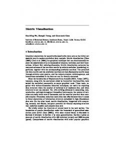
We use Iris data set as an example for showing the visualization of ensemble classifier. Fig. 5 shows four individual classifiers whose training error is below a pre-defined threshold 0.1. From the attribute-class value mapping bars (refer to [2]) in Fig. 6, it is easy to see that the most related attributes are pw and pl (i.e., petalwidth and petallength). That explains why four pairs of attributes (pl, pl), (pw, pl), (pw, pw), (pl, pw) can grow the best trees. pw pl sw sl

Figure 6. Attribute-class value mapping bars. There are 4 bars corresponding to 4 attributes. Each bar consists of 150 dots (150 examples in the set) where each dot represents an attribute value, and the 150 dots are sorted according to their attribute values. The dot color indicates the class label. It is apparent that the attributes pw and pl have strong correlation with the class.

5.2 Ensemble decision tree visualization on large data sets To handle large data sets, our basic method is again to use sampling technique. Currently we implement random sampling only. More sophisticated sampling algorithm that can help find decision trees as different as possible, given the number of trees, will be explored in the future. The purpose of this section is to see if it is effective to use simple random sampling with very small sample size.

To this end, we test the ensemble classifier on 5 Statlog data sets: Satimage, Segment, Shuttle, Australian, and DNA. For data description, please see Table 3. The reason to use these 5 Statlog data sets is because Ankerst used them as benchmark in his PBC system [2]. The experimental results in Table 4 show that even with very small sample size, the ensemble classification accuracy is comparable with PBC using complete training data set. And the average tree size of ensemble classifier using small sample is significantly smaller than PBC. For an example of ensemble classifier visualization on Satimage (satellite image) data, please refer to Fig.7.

Table 3. Data description of 5 Statlog data sets. For Segment and Australian, we use 10-fold cross-validation to evaluate the accuracy. For Satimage, Shuttle and DNA, the size only indicates that of the train set. There are separate test set for these three data sets. Dataset Satimage Segment Shuttle Australian DNA

size 4435 2310 43500 690 2000

classes 6 7 7 2 3

categorical 0 0 0 6 60

numerical 36 19 9 8 0

5.3 Discussion Though ensemble classifier visualization has the above advantages, there are several issues needed to mention. First, the number of different good trees might be huge.

Table 4. Comparison of accuracy and tree size of Ankerst’s PBC system and our ensemble algorithm using random sampling technique. The sample size is set to 100 and the number of individual classifiers in an ensemble is 9. Dataset Satimage Segment Shuttle Australian DNA

Accuracy PBC Ensemble 83.5 80.5 94.8 91.2 99.9 99.5 82.7 84.7 89.2 91.9

Tree size PBC Ensemble 33 6-7 21.5 7-8 8.9 4-5 9.3 5-6 18 7-8

For example, when there are lots of redundant or strongly correlated attributes, the number of different trees can be exponential to the number of related attributes. Digit recognition data set [10] is such an example. All seven attributes (horizontal and vertical lights in on-off combinations) are strongly related. In this case, we need alternative tools to help user understand why the tree structure might be so unstable. Pixel bar charts technique could be such a tool [20]. Second, we may need to have a measurement of the difference or distance of two tree structures. If two trees are slightly different according to the measurement, we would like to remove it from the ensemble and try to find a new different tree. The distance of two trees can be defined as the prediction error on a common test set. If the two trees are generated from different samples, we can use the union of the two samples as the test set. Third, having more than one trees implies that the organization of trees should be considered. One simple way is to set a priority for each attribute, and then apply some mechanisms such as sorting with combinatory attributes or fields. Another interesting approach might be to apply some clustering techniques to group similar trees together according to the definition of tree distance.

6 Summary and Future work Shaded similarity matrix is a visualization approach used in hierarchical cluster analysis. This paper takes the unified point on viewing classification and clustering (supervised and unsupervised learning) from some researchers [22, 18, 8]. This leads us to believe shaded similarity matrix can also be used in the task of classification visualization. In this paper, we investigated how shaded similarity matrix is used to visualize two popular classification methods: nearest neighbor and decision tree. We also explored a method to solve large data sets by using ensemble classification and sampling techniques.

This paper has not explored the following interesting issues. First, can weighted distance definition or nonlinear distance definition improve the grouping quality when using typical Euclidean distance failed to reveal the withinclass clusterings? And how to use visualization to help find a better distance definition? Second, can we design a sampling approach which can guarantee the convergence of an ensemble classifier whose individual classifiers satisfy some constraints such as the training error threshold? In other words, after a convergence point, taking more rounds of sampling will not change the ensemble. This seems to be a theoretical question related more to the (online) computational learning instead of visualization. However, the solution to this problem can provide users a more reliable ensemble classifier visualization.

Acknowledgments This work was partially supported by the Information Systems Research Lab (ISRL) of the Graduate School of Library and Information Science at University of Illinois at Urbana-Champaign. We are thankful to the Research Writing Group of ISRL directed by Dr. David Dubin.

References [1] M. Ankerst, C. Elsen, M. Ester, and H.-P. Kriegel. Visual classification: An interactive approach to decision tree construction. In Proceedings of the Fifth International Conference on Knowledge Discovery and Data Mining, pages 392–396, 1999. [2] M. Ankerst, M. Ester, and H.-P. Kriegel. Towards an effective cooperation of the user and the computer for classification. In Proceedings of the Sixth International Conference on Knowledge Discovery and Data Mining, pages 179–188, 2000. [3] S. T. Barlow and P. Neville. Case study: Visualization for decision tree analysis in data mining. In Proceedings of IEEE Symposium on Information Visualization 2001, pages 149–152, 2001. [4] S. T. Barlow and P. Neville. A comparison of 2-D visualizations of hierarchies. In Proceedings of IEEE Symposium on Information Visualization 2001, pages 131–138, 2001. [5] B. Becker. Visualizing decision table classifiers. In Proceedings of IEEE Symposium on Information Visualization 1998, pages 102–105, 1998. [6] B. Becker, R. Kohavi, and D. Sommerfield. Visualizing the simple bayesian classifier. In KDD Workshop on Issues in the Integration of Data Mining and Data Visualization, 1997. [7] T. Biedl, B. Brejova, E. Demaine, A. Hamel, and T. Vinar. Optimal arrangement of leaves in the tree representing hierarchical clustering of gene expression data. Technical report, Dept. of Computer Science, University of Waterloo, 2001.

[8] H. Blockeel, L. De Raedt, and J. Ramon. Top-down induction of clustering trees. In J. Shavlik, editor, Proceedings of the 15th International Conference on Machine Learning, pages 55–63. Morgan Kaufmann, 1998. [9] L. Breiman. Bagging predictors. Machine Learning, 24(2):123–140, 1996. [10] L. Breiman, J. Friedman, R. Olshen, and C. Stone. Classification and Regression Trees. Chapman & Hall, 1984. [11] A. Buja and Y.-S. Lee. Data mining criteria for tree-based regression and classification. In Proceedings of the Seventh International Conference on Knowledge Discovery and Data Mining, pages 27–36, 2001. [12] B. V. Dasarathy. Nearest Neighbor (NN) Norms: NN Pattern Classification Techniques. IEEE Computer Society Press, Los Alamitos, California, 1990. [13] Y. Freund and R. E. Schapire. Experiments with a new boosting algorithm. In Proceedings of the 13th International Conference on Machine Learning, pages 148–156, 1996. [14] N. Gale, W. Halperin, and C. Costanzo. Unclassed matrix shading and optimal ordering in hierarchical cluster analysis. Journal of Classification, 1:75–92, 1984. [15] http://www.angoss.com. [16] http://www.spss.com. [17] A. Inselberg and T. Avidan. Classification and visualization for high-dimensional data. In Proceedings of the Sixth International Conference on Knowledge Discovery and Data Mining, pages 370–374, 2000. [18] A. Kalton, P. Langley, K. Wagstaff, and J. Yoo. Generalized clustering, supervised learning, and data assignment. In Proceedings of the Seventh International Conference on Knowledge Discovery and Data Mining, 2001. [19] D. A. Keim and M. Ankerst. Visual data mining and exploration of large databases. In Proceedings of the 5th European Conference on Principles and Practice of Knowledge Discovery in Databases, Freiburg, Germany, 2001. [20] D. A. Keim, M. C. Hao, U. Dayal, and M. Hsu. Pixel bar charts: A visualization technique for very large multiattributes data sets. Information Visualization, 1, 2002. [21] R. Kohavi and D. Sommerfield. Targeting business users with decision table classifiers. In Proceedings of the Fourth International Conference on Knowledge Discovery and Data Mining, pages 249–253, 1998. [22] P. Langley. Elements of Machine Learning. Morgan Kaufmann Publishers, 1996. [23] R. L. Ling. A computer generated aid for cluster analysis. Communications of the ACM, 16(6):355–361, 1973. [24] R. Maclin and D. Opitz. An empirical evaluation of bagging and boosting. In Proceedings of the Fourteenth National Conference on Artificial Intelligence, pages 546–551. AAAI Press/MIT Press, 1997. [25] C. J. Merz, P. M. Murphy, and D. W. Aha. UCI repository of machine learning databases, http://www.ics.uci.edu/˜mlearn/mlrepository.html, 1997. Dept. of Information and Computer Science, University of California at Irvine. [26] T. Mitchell. Machine Learning. McGraw Hill, 1997. [27] F. Provost and V. Kolluri. A survey of methods for scaling up inductive algorithms. Data Mining and Knowledge Discovery, 2:1–42, 1999.

[28] R. E. Schapire. The boosting approach to machine learning: An overview. In MSRI Workshop on Nonlinear Estimation and Classification, 2002. [29] S. B. Thrun, J. Bala, E. Bloedorn, I. Bratko, B. Cestnik, J. Cheng, K. D. Jong, S. D. zeroski, S. E. Fahlman, D. Fisher, R. Hamann, K. Kaufman, S. Keller, I. Kononenko, J. Kreuziger, R. S. Michalski, T. Mitchell, P. Pachowicz, Y. Reich, H. Vafaie, W. V. de Welde, W. Wenzel, J. Wnek, and J. Zhang. The MONK’s problems: A performance comparison of different learning algorithms. Technical Report CS-91-197, School of Computer Science, Carnegie Mellon University, Pittsburgh, PA, 1991. [30] D. Wishart. ClustanGraphics3: Interactive graphics for cluster analysis. In W. Gaul and H. Locarek-Junge, editors, Classification in the Information Age, pages 268–275. SpringerVerlag, 1999.

Appendix A The purpose of this appendix is to show that when distance is defined only on class, within-cluster average distance is equivalent to the Gini index [10]. P ROOF. We consider only the two-class situation4 . The class labels are denoted 0 and 1. Given a split into left and right subsets, let p0L +p1L = 1, p0R +p1R = 1 be the probabilities of label 0 and 1 on the left and on the right, respectively. Denoting with pL + pR = 1 the probabilities of the left and the right subset given the parent data set. Then Gini index takes this form: Gini = pL p0L p1L + pR p0R p1R Now suppose the distance of two examples e1 and e2 is defined only on class information: ½ 0 if e1 and e2 share the same class δ(e1 , e2 ) = 1 otherwise Then the within-cluster average distance weighted on the left and right subsets can be written as: P P ei ,ej ∈SL δ(ei , ej ) ei ,ej ∈SR δ(ei , ej ) pL + pR 2 |SL | |SR |2 0 1 2|SR ||SR | 2|SL0 ||SL1 | + pR = pL 2 2 |SL | |SR | = ∝

2(pL p0L p1L + pR p0R p1R ) Gini

Where SL , SR denoting the left and right subset, respectively; and |SL0 |, |SL1 | denoting the number of examples with label 0 and 1 in the left subset, respectively; and so on.

4 Some

notations are taken from [11]


f13 < 77.5 [65] f30 < 66.5 [20]

f13 >77.5 [35]

f30 >66.5 [45]

f11 f11 f24 94.5 [13] 77.0 [40]

f14 >64.5 [43]

f3 f3 f16 91.5 [8] 59.5 [26]

2

21

f24 >104.5 [7]


f15 >87.5 [38]

0

f24 77.0 [32]

f14 81.0 [31]

f8 >74.0 [39]

0

8


f21 f21 61.5 [23]

f8 < 74.0 [30] f2 f2 65.0 [23]

2 1

f29 < 81.0 [69]

f22 < 92.5 [8] f22 >92.5 [27]

f24 >73.0 [27]

0

21


f4 < 77.0 [7] f4 >77.0 [33]

f16 >73.5 [26]

2

16

1

25

4

8

3

(d)

Figure 7. Ensemble decision tree visualization on Satimage data.

30

11 5 10

mammal

reptile

41

bird

20

amphibian invertebrate

5 fish 13

4 insect 8

10

a) k-nearest neighbor setting: k=7

mammal

reptile

41

bird

20

5 fish 13

amphibian invertebrate

4 insect 8

10

b) Distance threshold setting: Threshold=0.4

Figure 8. Two different control settings on whether to display a matrix cell or not.

a) Distance threshold = 0.1

b) Distance threshold = 0.3

Mammal [41] ostrich Bird [20] Reptile [5]

Fish [13] Amphibian [4]

Insect [8]

Invertebrate [10]

c) Distance threshold = 0.5

d) Distance threshold = 0.7

Figure 9. Gradually increasing the distance threshold shows how the regularities and outliers emerge.