Qualitative Polyline Similarity Testing with Applications to Query-by-Sketch, Indexing and Classification Bart Kuijpers
Bart Moelans
Nico Van de Weghe
Theoretical Computer Science Hasselt University & Transnational University of Limburg, Belgium
Theoretical Computer Science Hasselt University & Transnational University of Limburg, Belgium
Geography Department Ghent University B-9000 Ghent, Belgium
[email protected] [email protected] ABSTRACT We present an algorithm for polyline (and polygon) similarity testing that is based on the double-cross formalism. To determine the degree of similarity between two polylines, the algorithm first computes their generalized polygons, that consist of almost equally long line segments and that approximate the length of the given polylines within an ε-error margin. Next, the algorithm determines the double-cross matrices of the generalized polylines and the difference between these matrices is used as a measure of dissimilarity between the given polylines. We prove termination of our algorithm and “ show that its sequential time complexity is ” max(N1 ,N2 ) 2 ) , where N1 and N2 are the bounded by O ( ε number of vertices of the given polylines. We apply our method to query-by-sketch, indexing of polyline databases, and classification of terrain features and show experimental results for each of these applications.
Categories and Subject Descriptors H.2.1 [Database Management]: Logical Design; H.2.8 [Database Management]: Database Applications—Spatial databases and GIS
General Terms Algorithms, Theory, Design
Keywords Polygons, Polylines, Similarity, Double-Cross Calculus, Qualitative Calculi
1.
INTRODUCTION AND SUMMARY
In several domains, such as computer vision, image analysis and GIScience, shape recognition and retrieval are central
Permission to make digital or hard copies of all or part of this work for personal or classroom use is granted without fee provided that copies are not made or distributed for profit or commercial advantage and that copies bear this notice and the full citation on the first page. To copy otherwise, to republish, to post on servers or to redistribute to lists, requires prior specific permission and/or a fee. ACM-GIS’06, November 10–11, 2006, Arlington, Virginia, USA. Copyright 2006 ACM 1-59593-529-0/06/0011 ...$5.00.
[email protected]
problems. Roughly speaking, there are two approaches to shape recognition and retrieval: the quantitative approach and the qualitative approach. Traditionally, most attention has gone to the quantitative methods [?, ?, ?, ?] and only recently, the qualitative approach has gained more attention, supported by cognitive studies that provide evidence that qualitative models of shape representation tend to be much more expressive than their quantitative counterpart [?]. It is widely accepted that shapes are one of the most complex phenomena that have been dealt with using a qualitative representation of space [?]. Within the qualitative approaches to describe two-dimensional shapes there are two major approaches: the regionbased and the boundary-based approach. The region-based approach uses global properties such as circularity, eccentricity and axis orientation to describe shapes. As a result, this approach can only discriminate shapes with large dissimilarities [?]. The boundary-based approach describes the type and position of localized features (such as vertices, extremes of curvature and changes in curvature) along the polyline representing the shape [?]. Among the boundary-based approaches are [?, ?, ?, ?, ?, ?, ?]. In this paper, we assume shapes to be described by their boundaries, which we assume to be polygons. As a generalization of polygons, we consider polylines and use this more general term in the remainder of the exposition, also to include polygons. At the basis of polyline recognition and retrieval lie algorithms to determine similarity between polylines. Here, we follow the qualitative formalism provided by the double-cross calculus [?, ?], which is used in the qualitative trajectory calculus for shapes [?], to test for polyline similarity. The double-cross matrix of a polyline contains for each pair of line segments in the polyline a 4-tuple of −, +, and 0 that describes the relative qualitative position of these line segments to each other. We remark that there are 81 possible such 4-tuples, but that only 65 of these 4-tuples are physically realizable. For two given polylines, our method computes, if the polylines have equally many vertices, the double-cross matrices of the polylines and returns some distance value between these matrices as a measure of dissimilarity. A problem might be that the two given polylines of which we want to test similarity, may be given with a different number of vertices. To overcome this difference, our algorithm first computes for each of the two polylines a series of so-called generalized polylines, that consist of 2, 4, 8, ..., 2n , ... line segments.
The nth generalizednpolyline has its vertices exactly at fractions 0, 21n , 22n , ..., 22n of the length of the original polyline. The generalized polylines have the property that they converge (also in length) to the given polylines and that they tend to consist of equally long line-segments. The latter property has the advantage that line segments analogously subdivided polylines, point to relatively analogous places on the polylines. The idea of using generalized polylines was introduced by two of the present authors in [?] and used in a naive way. In this paper, we optimize this approach and give a theoretical analyzis and complexity considerations of this idea. Our algorithm for testing the similarity of two polylines, given by a sequence of vertices, works grosso modo as follows. For two given polylines, the algorithm computes their respective generalized polylines until their lengths approximate that of the given polylines sufficiently (this is formalized by an error-percentage ε that is part of the input). Once we have the generalized polylines, we compute their double-cross matrices and output the distance between these matrices. There are many possible ways to define a distance function between matrices. The one that we discuss in this paper, has shown to give the best results in practical experiments. To compute this distance, we first create for each of the two double-cross matrices a 65-ary vector of natural numbers that counts for each of the 65 realizable 4-tuples of −, + and 0, the number of times they occur in the matrix. The distance-function then counts the average difference between the 65 count values. We prove several properties of our algorithm for testing polyline similarity. The algorithm is guaranteed to terminate on any input and when it terminates the generalized polyline tends to consist “ of equally”long line segments. It computes at most ⌊log max(Nε 1 ,N2 ) ⌋ + 1 generalized polylines, where N1 and N2 are the number of vertices of the given polylines. We also show a theoretical upper bound on the overall ” complexity of our algorithm, “ sequential time which is O ( max(Nε 1 ,N2 ) )2 . Although our algorithm contains large parts that are parallellizable, this only gives a gain by a factor of 2 compared to the sequential time complexity. We apply our algorithm to three problems and give empirical test results on geographic data. Firstly, we consider the problem of similar polygons. We apply our implementation to various (polygonalized) sketches of a map of Belgium and it correctly orders the sketches in terms of increasing similarity. Secondly, we take a look at the query-by-sketch problem, which allows a user to visually describe shapes or movements, in order to retrieve them from a database [?, ?]. It turns out that our algorithm performs well in classifying sketches of maps and also in retrieving geographic data given a query that is expressed as a two-dimensional sketch. In this experiment we also show the above mentioned 65dimensional vector of count values can be used as an index on a database containing polygonal figures. We consider the problem of retrieving cities in Belgium by sketch and the output, which is a top 4 of best fitting cities, seems to correspond to what the human eye would recognize. Thirdly, we apply our algorithm to polylines that represent terrain features (such as plateau, mesa, flat-floored valley, u-shape valley, depression and canyon) [?]. Experiments
on fairly simple terrains give good results, but it seems that for more complex profiles, a division is needed according to the local maxima or minima of the terrain to obtain fits for the corresponding parts of the terrain. Organization. This paper is organized as follows. In Section ??, we define polylines and generalized polylines. Also the double-cross formalism is explained there. In Section ??, the algorithm for testing polyline similarity is given and some basic properties are proven. We also give an analysis of its computational complexity. In Section ??, we discuss the experiments with query-by-sketch, indexing and classification of terrain features.
2. DEFINITIONS AND PRELIMINARIES In this section, we define polylines and generalized polylines and explain the double-cross formalism.
2.1 Polylines and polygonal shapes Let R denote the set of real numbers and R2 the real plane. Definition 1. A polyline P in R2 is a piecewise linear curve that is given by an ordered list of its vertices, i.e., P = h(x0 , y0 ), (x1 , y1 ), ..., (xN , yN )i. A polygonal shape (or polygon) is a polyline P = h(x0 , y0 ), (x1 , y1 ), ..., (xN , yN )i for which (x0 , y0 ) = (xN , yN ). Let P = h(x0 , y0 ), (x1 , y1 ), ..., (xN , yN )i be a polyline. The vertices (x0 , y0 ) and (xN , yN ) are respectively the start and end vertex of P . We denote the line segment between (xi , yi ) and (xi+1 , yi+1 ) by Li (P ) and its length by ℓ(Li (P )). We call ℓ(P ) := ℓ(L0 (P )) + ℓ(L1 (P )) + · · · + ℓ(LN−1 (P )) the length of P . The vector from (xi , yi ) to (xi+1 , yi+1 ) will be → − denoted ℓi (P ). If P is clear from the context, we will omit (P ) from the above notations. The semantics of the polyline P = h(x0 , y0 ), (x1 , y1 ), ..., (xN , yN )i is the subset of R2 consisting of all line segments between consecutive vertices of P , and we write [ Li (P ). sem(P ) := 1≤i 0 when θ ∈]−90◦ , 90◦ [, so when → u .→ v > 0. → − → − ◦ ◦ And finally u . v < 0 is equivalent to θ ∈]90 , 270 [. When → − → − − − we apply this reasoning to → v = ℓ′i and → v = ℓ′j , we obtain → − − the expressions for C1 and C2 : C1 = −sign(→ u · ℓ′i ) and → − − C2 = −sign(−→ u · ℓ′j ). → − − − For C3 , we consider the block-product (→ u × ℓ′i ) · → w . This → − − product is zero if and only if → u and ℓi are collinear. The − vectorial product → u × ℓ~′i is a vector pointing in the direction → − of positive z-coordinate if and only if ℓ′i is on the right of → − → − − − u , which means that (→ u × ℓ′j ) · → w < 0 in this case. The case of C4 is completely similar to that of C3 , after − interchanging left and right. So, we have C3 = −sign((→ u × → −′ → → − − → − → − ′ ℓ ) · w ) and C = sign(( u × ℓ ) · w ). i
4
j
→ − → − The following property says how DC( ℓj , ℓi ) can be de→ − → − rived from DC( ℓi , ℓj ) in a straightforward way. → − → − Proposition 2. If DC( ℓi , ℓj ) = (C1 C2 C3 C4 ), then we → − → − have DC( ℓj , ℓi ) = (C2 C1 C4 C3 ). If we write −− for +; −+ for − and −0 for 0, we easily obtain the following property. → − → − Proposition 3. If DC( ℓi , ℓj ) = (C1 C2 C3 C4 ) and σ : R2 → R2 is a reflection along a line, then we have the equal→ − → − ity DC(σ( ℓi ), σ( ℓj )) = (C1 C2 − C3 − C4 ).
2.3 The double-cross matrix DCM Based on the double-cross formalism, we now define the double-cross matrix of a polyline. Definition 4. A double-cross matrix DCM (P ) of a polyline P = h(x0 , y0 ), (x1 , y1 ), ..., (xN , yN )i is a N × N matrix → − → − with DCM (P )[i, j] = DC( ℓi , ℓj ). Because of Proposition ?? and because the diagonal entries of DCM (P ) are all (0 0 0 0), it suffices to consider only 2 the upper triangle of the matrix DCM (P ), i.e., the N 2−N elements DCM (P )[i, j] with i < j. The following property is easily verified. Proposition 4. Let P be a polyline and let α : R2 → R2 be an orientation-preserving isometry (i.e., a composition of a rotation and translation) or a point-scaling (i.e., a mapping of the form (x, y) 7→ a · (x, y) with a 6= 0, then DCM (P ) = DCM (α(P )). We remark that the double-cross matrix is not invariant under scalings of the form (x, y) 7→ (a · x, b · y) with a 6= b. More specifically, C1 and C2 are not invariant under these scalings, but C3 and C4 are invariant.
3. POLYLINE SIMILARITY ALGORITHM 3.1 The algorithm DC-similar∆ We now describe our algorithm for determining the similarity of polylines and polygonal shapes (we give it in pseudocode). This algorithm returns a degree of similarity between two given polylines P1 and P2 . It uses an error rate ε (with 0 ≤ ε ≤ 1) and depends on a distance function ∆ between double-cross matrices, which we consider a parameter of the algorithm. Basically, the algorithm computes the generalized polylines of P1 and P2 until these approximate the length of P1 and P2 up to an error ε (a “small” percentage of the length). Then the double-cross matrices of the generalized polylines are computed and the distance between them is returned. Algorithm DC−similar ∆ input : t r a j e c t o r i e s P1 , P2 ; threshold 0 ≤ ε ≤ 1 . set n : = 1 ; compute P12 and P22 ; n
while |ℓ(P12 ) − ℓ(P1 )| ≥ ε · ℓ(P1 ) n o r |ℓ(P22 ) − ℓ(P2 )| ≥ ε · ℓ(P2 ) do n:=n+1; compute i n p a r a l l e l n n−1 1 . P12 from P12 and P1 ; and n n−1 2 . P22 from P22 and P2 ; od compute i n p a r a l l e l n 1 . M1 := DCM (P12 ) ; and n 2 . M2 := DCM (P22 ) ; return ∆(M1 , M2 ) . As mentioned, ∆(M1 , M2 ) expresses a measure of difference or distance between the two double-cross matrices M1 and M2 . There are many possibilities here, but in our experiments we have used the distance function ∆H (for an alternative function ∆E , we refer to Section ??). To define the distance measure ∆H (M1 , M2 ) between DoubleCross matrices, we first construct, for both matrices M1 and M2 , vectors γ(M1 ), γ(M2 ) ∈ N65 that counts for each of the 65 realizable 4-tuples of −, + and 0, the number of times they occur in the matrices M1 and M2 . Then ∆H (M1 , M2 ) =
N2
65 X 1 |γ(M1 )[i] − γ(M2 )[i]| . − N i=1
The function ∆H counts the average difference between the 65 count values.
3.2 Basic properties of DC-similar∆ We now give some basic properties of DC-similar∆ . To start, we show that the algorithm is guaranteed to terminate on any input. We remark that these properties are independent of the choice of ∆ (as long as the evaluation of ∆ terminates). Proposition 5. The algorithm DC-similar∆ terminates on any inputs P1 , P2 and 0 < ε ≤ 1.
Proof. To prove this property, it suffices to show that for any polyline P andn any 0 < ε ≤ 1, there exists an n ≥ 1 such that |ℓ(P ) − ℓ(P 2 )| < ε · ℓ(P ). We prove this by showing n that limn→∞ ℓ(P 2 ) = ℓ(P ). n+1 n If we construct P 2 from P 2 and P there are two posn+1 sibilities: (1) if each vertex of P 2 is also an element n n of sem(P 2 ), then sem(P 2 ) = sem(P ) and thus ℓ(P ) = n n+1 ℓ(P 2 ) = ℓ(P 2 ) and the stop condition is satisfied; (2) n+1 there is at leastnone vertex p of P 2 that is not an ele2 ment of sem(P ). Because of the triangle inequality and n n+1 by construction we know that ℓ(P 2 ) < ℓ(P 2 ) ≤ ℓ(P ). n From these two cases we can deduce that limn→∞ ℓ(P 2 ) = ℓ(P ) and therefore there exists an n ≥ 1 such that |ℓ(P ) − n ℓ(P 2 )| < ε · ℓ(P ).
(a)
(b)
(c)
(d)
Proposition 6. When the algorithm DC-similar∆ , on input P1 , P2 and 0 < ε ≤ 1, terminates for some n, then then standard deviation of the lengths of the line segments of Pk2 tends to 0, more specifically, it is bounded by 2εn · ℓ(Pk ) (k = 1, 2). Proof. Let P be P1 or P2 and let L1 , ..., L2n be the line n segments of P 2 . Let ℓ¯ denote the average length of the segments L1 , ..., L2n . The square of the standard deviation P n ¯ 2 . By construction and the σ is then 21n 2i=1 (ℓ(Li ) − ℓ) ) . We also triangle inequality we know that ℓ(Li ) ≤ ℓ(P 2n n P n 2 2 know that ℓ(P ) = i=1 ℓ(Li ) > ℓ(P ) · (1 − ε). Therefore P n ) ) σ 2 ≤ 21n 2i=1 ( ℓ(P − ℓ(P )(1−ε) )2 = ( ℓ(P · ε)2 and thus σ ≤ 2n 2n 2n ε · ℓ(P ). 2n
3.3 Time complexity of DC-similar∆H The following property gives an upper bound for the sequential time complexity of DC-similar∆H . We remark, that although large parts of DC-similar∆H can be performed in parallel, this only gives a gain of a factor of 2. Proposition 7. The algorithm DC-similar∆H , on input P1 = h(r0 , s0 ), (r1 , s1 ), ..., (rN1 , sN1 )i, P2 “= h(u0 , v0 ), (u1”, v1 ), ..., (uN2 , vN2 )i and 0 < ε ≤ 1, needs O ( max(Nε 1 ,N2 ) )2 sequential time to return its output.
Proof. Let P = h(x0 , y0 ), (x1 , y1 ), ..., (xN , yN )i be P1 or n P2 . The difference between P and P 2 is that line segments n of P 2 can short cut angles of P . Such a short-cut angle ) and there can at (or series of angles) of P has length ℓ(P 2n most be N cut angles. The difference in length between P n ) and P 2 is therefore bounded by N · ℓ(P . We remark that 2n this number will eventually, for increasing n, become smaller than ε · ℓ(P ), since N.ℓ(P ) is fixed. Therefore, the algorithm DC-similar∆H terminates, on input P1 and P2 , as soon as 2) 1) < ε · ℓ(P1 ) and N2 · ℓ(P < ε · ℓ(P2 ). This is true N1 · ℓ(P 2n 2n `M ´ for n = ⌊log ε ⌋ + 1 with M = max(N1 , N2 ). In this case, the while-loop of the algorithm has calculated maximally M 2⌊log( ε )⌋+1 ≤ 2 M vertices on the generalized polylines and ε to compute the matrices M1 and M2 in the algorithm, we )2 −2 M (2 M ε ε 2
≤ 2.( M )2 entries. need in worst cast to calculate ε The function ∆H just scan each tuple of M1 and M2 in parallel once and needs maximum O( M ) sequential time. ε
(e) Figure 4: A map of Belgium and some sketches.
4. EXPERIMENTAL RESULTS In this section we discuss three experiments using Javaimplementations of the algorithm DC-similar∆H . The run time results we mention are with respect to a system with r r 1.86 GHz processor and 1GB RAM an Intel Pentium
M running Kubuntu as operating system.
4.1 Experiment 1: Polygon similarity For the first experiment, we used five figures representing Belgium (see Figure ??). Figure ?? is the correct representation of Belgium, consisting of 2047 line segments. Figure ?? is the same figure with the three bumps in the upper part moved to the right. The remaining three figures are sketches of Belgium made by respectively a geographer (Figure ??: real representation, Figure ??: abstract representation) and a non-specialist (Figure ??). Figure ?? ?? ?? ?? ?? ?? 100% 99% 87% 66% 60% ?? 100% 87% 67% 60% ?? 100% 80% 69% ?? 100% 84% ?? 100% Table 1: Similarity between polygons of Figure ?? using ∆H with threshold 5%. We applied the algorithm DC-similar∆ for ∆ = ∆H to each two of these five figures with a threshold ε = 5%. The result are given in Table ??. The measure ∆H gives results that are very much in line with our intuition. For the above mentioned hardware, ∆H takes ±2.5 minutes to calculate the similarity of 2 shapes with 215 line-segments (so ±229 entries). These experiments are in line with the theoretical
complexity bound given by proposition ??. Figure ??, with the three bumps moved to the right is 99% similar to the real map. The remaining three sketches of Belgium are ordered with decreasing similarity corresponding to our feeling. We remark that ∆H , because it is based on counting entries in the double-cross matrices, gives the same result, independent of the start vertex of polygonal input figures.
4.2 Experiment 2: Query by sketch
Figure 6: Bowler hat and bow tie sketch.
Because several experiments indicated that ∆H gives good, start-vertex-independent results, we used the vector of 65 count values that is constructed by ∆H as a method to index a database. This index is then used to support query-bysketch. The 65-ary vector for a sketched figure is computed and, e.g., the four figures in the database that have a 65-ary vector closest to it are returned in order of descending best match.
Figure 7: Result of bowler hat query (dark gray) and bow tie query (light gray).
the most as the bow tie sketched on the right in Figure ??.” The resulting cities are colored light gray in Figure ??. The best fit is the village at the bottom right. Figure 5: The 43 cities and villages of Limburg. More precisely, we have applied this method to perform a query-by-sketch on the villages and cities of Belgium. In this experiment we have calculated these index value for villages and cities, such that the generalized polygons of all cities approximate the length of the original polygon with an error smaller than 2%. Then for each of the villages and cities the 65-ary vector with count values of the 65 possible 4-tuples of −, + and 0, is calculated as an index. Next, we queried for the presence of a sketched village. The sketched polygon is generalized up to the same level as the cities and villages in the database are; its index value is computed; and the four best fits (using the distance given by ∆H ) are returned. For the sake of producing readable figures, we here given an example of a query on a limited sample of cities in Belgium, namely the villages and cities in the province of Limburg, as depicted in Figure ??. This province consists of 43 villages and cities and it is not connected. Building the index for this sample has costed 0.8 seconds on the abovementioned configuration. The first query is: “Give the 4 cities of Limburg looking the most as the bowler hat sketched on the left in Figure ??.” The resulting cities are colored dark gray in Figure ??, with Lommel, the most similar city, shown in the north. We remark that Proposition ?? guarantees that similarity is tested invariantly under translations, rotations and scalings, as can be seen from these results. Indeed, Lommel, looks like a the given bowler hat but 45◦ rotated. Another query was: “Give the 4 cities of Limburg looking
4.3 Experiment 3: Classification of terrain features Our last experiment deals with terrain features.The figures in this experiment are inspired by work of Kulik and Egenhofer [?]. We used the seven figures in Figure ?? as primitive terrain features to classify some silhouettes of terrains. We use our ∆H measure to classify the figures in Figure ??. Our ∆H algorithm classifies the three silhouettes of Figure ??, as (a) Mesa, (b) U-Valley and (c) Mesa (or U Valley) respectively (see Tables ??,?? and ??). For (a) and (b) this corresponds to our visual observations. Figure ?? (c) is more complicated and needs more attention. We divided this figure according to its local maxima and minima (see Figure ??). The resulting classifications, summarized in Tables ?? and ??, give a more precise description of these terrains.
Butte Plateau Mesa Flat Valley U Valley Depression Canyon
Fig. ?? 58% 62% 71% 48% 63% 47% 42%
Fig. ?? 52% 62% 64% 56% 77% 49% 50%
Fig. ?? 58% 64% 70% 50% 68% 50% 43%
Table 2: Classification by ∆H of Figure ?? using the primitives sketched in Figure ??.
(a) Butte
(b) Plateau
(c) Mesa (a)
(d) Flatfloored Valley
(e) U-shape Valley
(f) sion
(b)
Depres(c) Figure 9: Some silhouettes of terrains.
(g) Canyon Figure 8: Basic shapes of terrain features.
Butte Plateau Mesa Flat Valley U Valley Depression Canyon
A 67% 49% 68% 40% 48% 38% 39%
B 62% 58% 71% 40% 54% 41% 42%
C 68% 57% 78% 44% 56% 42% 40%
D 71% 40% 65% 46% 40% 30% 30%
E 52% 62% 62% 38% 49% 54% 47%
Table 3: Classification by ∆H of Figure ?? using the primitives sketched in Figure ??.
5.
DISCUSSION
We have given a number of basic properties and described the time complexity of the algorithm DC-similar∆ for testing polyline similarity. This algorithm depends on a function ∆ that measures the difference between double-cross matrices. We have experimented with a number of ∆’s and ∆H , used throughout the paper gives the best experimental results. As stated, one reason for this might be that it is independent from the choice of start vertex of a polygon. For polylines, that are not polygons, it might be preferable to work with a ∆ that compares corresponding line segments in the two polylines more directly. We here give an example of a ∆, namely ∆E , that is more appropriate for polylines. First, we define a distance δ between elements of {−, 0, +}: δ(−, −) := δ(+, +) := δ(0, 0) := 0, δ(−, 0) := δ(+, 0) := 1, δ(−, +) := 2 and δ(x, y) := δ(y, x). Next, we define a distance δ¯ between entries of the double-cross matrices: ¯ 1 C2 C3 C4 ), (C1′ C2′ C3′ C4′ )) δ((C
:=
4 X
δ(Ci , Ci′ ).
i=1
Finally, if P1 and P2 are polylines with N edges, then we define ∆E (DCM (P1 ), DCM (P2 )) :=
Butte Plateau Mesa Flat Valley U Valley Depression Canyon
a 52% 50% 53% 71% 54% 43% 31%
b 49% 40% 49% 54% 63% 43% 37%
c 49% 48% 53% 45% 61% 41% 52%
d 57% 41% 53% 62% 69% 34% 54%
e 52% 50% 53% 71% 68% 46% 43%
f 58% 66% 68% 47% 56% 56% 50%
Table 4: Classification by ∆H of Figure ?? using the primitives sketched in Figure ??. 1 4(N − 1)2
X
¯ δ(DCM (P1 )[i, j], DCM (P2 )[i, j]).
1≤i