A Model for Generating Random Quantified Boolean Formulas Hubie Chen Departament de Tecnologia Universitat Pompeu Fabra Barcelona, Spain
[email protected] Abstract The quantified boolean formula (QBF) problem is a powerful generalization of the boolean satisfiability (SAT) problem where variables can be both universally and existentially quantified. Inspired by the fruitfulness of the established model for generating random SAT instances, we define and study a general model for generating random QBF instances. We exhibit experimental results showing that our model bears certain desirable similarities to the random SAT model, as well as a number of theoretical results concerning our model.
1 Introduction A phenomenal success story of artificial intelligence research over the past decade has been progress on the boolean satisfiability (SAT) problem. The technology of solvers for SAT has been transformed by techniques such as conflict-driven learning, highly efficient propagation mechanisms, and randomization. Today, state-of-the-art solvers can cope with problem instances having sizes that are orders of magnitude beyond what one would have optimistically predicted a decade ago. Inspired and encouraged by the tremendous advances in boolean satisfiability, many researchers have recently turned to studying a powerful generalization of boolean satisfiability where both universal and existential quantification of variables is permitted; this generalization is often called the quantified boolean formula (QBF) problem. Whereas the SAT problem provides a framework wherein one can model search problems within the complexity class NP, the QBF problem permits the modelling of problems having higher complexity–from the complexity class PSPACE–including problems from the areas of verification, planning, knowledge representation, game playing, logic, and combinatorics. Recall that SAT is known to be NP-complete, and QBF is known to be PSPACE-complete. A significant tool for SAT research has been the model for generating random SAT instances studied by [Mitchell et al., 1992], in which it is possible to reliably generate instances that are robustly difficult. This model has become a canonical benchmark for solver evaluation, has been used heavily in conducting and thinking about SAT-related research, and is widely regarded as a suitable basis for investigating
Yannet Interian Center for Applied Mathematics Cornell University Ithaca, New York, USA
[email protected] “average” or “typical” case complexity. In addition, theoretical issues concerning this model have stimulated fruitful and highly non-trivial interaction among the areas of artificial intelligence, theoretical computer science, probability theory, and statistical physics. One particular question that has garnered significant attention is the “satisfiability threshold conjecture” which roughly states that, as the density of constraints is increased, formulas abruptly change from being satisfiable to being unsatisfiable at a critical threshold point. The utility and widespread embrace of the random SAT model suggests that research on QBF could similarly benefit from random QBF models. This paper defines and studies a general model for generating random instances of the QBF problem. We exhibit experimental results showing that our model bears certain desirable similarities to the random SAT model; in particular, we show that our model exhibits threshold and easy-hard-easy phenomena as in the SAT model. However, we also experimentally demonstrate that the much larger parameter space of our model offers a richer framework for exploring and controlling complexity than the SAT model. In addition, we present a number of theoretical results concerning our model, namely, we give techniques for establishing lower and upper bounds on the purported threshold in our model. This places our work in contrast to previous work on random QBF models (discussed below), which contained very little rigorous theoretical analysis. Our theoretical results demonstrate nice connections to both previously studied problems as well as less studied but natural problems; we believe that these results evidence that our model is mathematically tangible and holds promise for being analyzed on the level of sophistication that work on the SAT model has reached. Formulation of QBF. In this paper, we use the formulation of QBF where consecutive variables having the same quantifier are combined into a set. The following are the thus the general forms of QBF formulas having one, two, and three quantifier blocks, respectively: ∃X1 φ ∀Y1 ∃X1 φ ∃X2 ∀Y1 ∃X1 φ By a quantifier block, we mean an expression QV where Q is a quantifier (∃ or ∀) and V is a set of boolean variables. In
general, an instance of QBF contains a sequence of quantifier blocks which alternate between universal and existential type, followed by a set of clauses, denoted here by φ.1 The semantics of these formulas are defined as is standard in logic; for instance, a formula ∀Y1 ∃X1 φ is true if for every assignment to the variables Y1 , there exists an assignment to the variables X1 such that φ is true. An intuitive way to view a QBF formula is as a game between two players: a “universal player”, who attempts to falsify φ, and an “existential player”, who attempts to satisfy φ. Players set their variables in the order given by the quantifier prefix. For instance, a formula ∃X2 ∀Y1 ∃X1 φ can be viewed as a three-round game in which the existential player first sets the variables X1 , the universal player then sets the variables Y1 , and the existential player finishes by setting the variables X1 . In general, the formula is true if the existential player can always win the game by satisfying φ. Description of model. Let us review the random SAT model, which our model generalizes. This model takes three parameters: the clause length k, the number of variables n, and the number of clauses C. A random formula with these parameters, denoted here by k-F(n, C), is generated one clause at a time; each clause is generated by selecting, uniformly at random, k distinct variables, and then negating each with probability one half. Now we describe our random QBF model. In the random SAT model, every clause has the same length. In our model, this also holds, but in addition, the number of literals in a clause from each quantifier block is a constant. The first parameter to our model is thus a tuple specifying, for each quantifier block, the number of literals from that block that are in a clause. For instance, the tuple (2, 3) specifies that the generated formulas are of the form ∀Y1 ∃X1 φ, where each clause in φ has 5 literals, 2 from Y1 and 3 from X1 . We will call such formulas (2, 3)-QBF formulas. As another example, the tuple (4, 2, 3) specifies that the generated formulas are of the form ∃X2 ∀Y1 ∃X1 φ, where each clause in φ has 9 literals, 4 from X2 , 2 from Y1 , and 3 from X1 . Analogously, we call such formulas (4, 2, 3)-QBF formulas. The second parameter to our model is a tuple of the same length as the first one, specifying the number of variables in each quantifier block. The third parameter to our model is simply the number of clauses C. As an example, suppose that the first tuple is (2, 3), the second tuple is (44, 37), and the number of clauses is 290. The generated formulas are of the form ∀Y1 ∃X1 φ, where Y1 has 44 variables, X1 has 37 variables, each clause in φ has 2 literals from Y1 and 3 literals from X1 , and there is a total of 290 clauses in φ. Each clause is generated by selecting uniformly at random, for each quantifier block, the designated number of distinct variables, and then negating each variable with probability one half. We denote such a random formula by (2, 3)-F((44, 37), 290). In general, to denote random formulas from our model, we use 1 Note that we use the standard assumption that the innermost quantifier block is existential, for if it is universal, the block can be efficiently eliminated. We also assume, as usual, that different quantifier blocks have disjoint variable sets.
the notation (jl , kl , . . . , j1 , k1 )-F((ml , nl , . . . , m1 , n1 ), C) or (kl , jl−1 , . . . , j1 , k1 )-F((nl , ml−1 , . . . , m1 , n1 ), C) depending on whether or not the number of quantifier blocks is even or odd, respectively. Notice that in a random QBF from this model, if any quantifier block is picked and the clauses are restricted to literals over the quantifier block, the result is a random formula over the variables of the quantifier block in the sense of the random SAT model. It can in fact be verified that the model has a certain “recursive” property: generating a random QBF and then randomly instantiating the variables of the outermost quantifier block results in another random QBF from the model. Previous work. Random QBF models have been previously studied by [Cadoli et al., 1999] and [Gent and Walsh, 1999]. [Cadoli et al., 1999] have experimentally studied the QBF generalization of the SAT model where clauses of fixed length k are generated by randomly choosing k distinct variables from the entire set of variables, and then negating each with probability one half. In this generalization, denoted FCL, the generation of clauses does not differentiate among variables from different quantifier blocks. It was pointed out in [Gent and Walsh, 1999] that this model is “flawed” in that it generates trivially false formulas when the number of clauses is on the order of the square root of n, the number of variables. These trivially false formulas arise from pairs of clauses where one clause contains a single existential literal, the other contains a single existential literal that is the complement of the first, and no universal variable is repeated in the pair. In attempts to remedy this issue, [Gent and Walsh, 1999] proposed two models, model A and model B, and [Cadoli et al., 1999] proposed another model, FCL2. Model A and FCL2 are essentially modifications of the original FCL model that disallow the types of clauses that lead to the trivial falsity; for instance, in Model A, each clause is generated independently as before, but clauses containing one existential literal are simply discarded and replaced. As pointed out in [Gent and Walsh, 1999], instances generated by Model A lack uniformity; in our view, the definitions of Model A and FCL2 have an ad hoc flavor that we believe make them less amenable to mathematical analysis. The study of model B in [Gent and Walsh, 1999] is concerned mostly with QBF formulas with two quantifier blocks; results of two experiments are reported. The parameterizations of Model B studied can be obtained within our model, and indeed our model can be viewed as a generalization of these parameterizations. However, no systematic definition of the parameter space of Model B is given. We believe that one of the contributions of this paper is the precise articulation of a general random QBF model that may be instantiated in various ways, and from which it is possible to methodically embark on experimental and theoretical explorations of the parameter space.
6e+08 rho 1.2 rho 1.0 rho 0.8 rho 0.6
number of branches
5e+08
4e+08
3e+08
2e+08
1e+08
0 6
6.5
7
7.5
8
8.5
9
9.5
10
10.5
11
ratio=clauses/(existential variables)
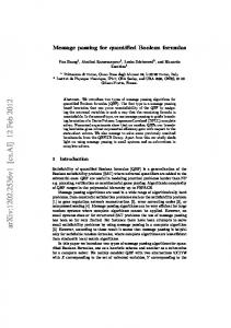
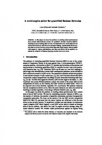
Figure 1: Computational cost of random (2, 3)-QBF formulas with 80 variables. Each curve corresponds to a different value of ρ. For instance, using the introduced notation, the curve with ρ = 0.6 corresponds to the hardness of formulas of the form (2, 3)-F((30, 50), C) for varying numbers of clauses C. The hardness is plotted as a function of the ratio of clauses to existential variables; in the case of ρ = 0.6 and 80 variables, this ratio is equal to C/50. Note that all of the experiments were performed using the solver QuBE-BJ [Giunchiglia et al., 2001], and each point of our plots represents the median value. Figure 2 concerns exactly the same formulas studied by Figure 1, but shows the probability of truth instead of the computational cost. 1 rho 1.2 rho 1.0 rho 0.8 rho 0.6
probability sat
0.8
3.5e+07
1 3 alt prob
3e+07
2.5e+07
2e+07 0.5 1.5e+07
probability sat
Our first set of experimental results concerns (2, 3)-QBF formulas, all of which have the same number of variables, 80. We varied both the number of clauses, as well as the ratio of universal to existential variables, denoted by ρ (rho). Figure 1 shows the computational cost of deciding these formulas.
this transition seems to take place relatively abruptly, suggesting that our model exhibits a threshold phenomenon as is conjectured in the random SAT model. Also, recall that in the random SAT model, computational difficulty exhibits an easy-hard-easy pattern, where the computational difficulty of formulas peaks around the point where half of the forulas are satisfiable. For each value of ρ in these two figures, and in all of the other experiments we performed, our model also exhibits this phenomena. Now, let us consider the curves of Figure 1 together. The picture suggested is an extremely intriguing one: starting from the left, the peaks of each of the four curves appear to increase as ρ decreases, attain a maximum, and then decrease as ρ further decreases. That is, the peaks of the easy-hardeasy patterns appear to themselves exhibit an easy-hard-easy pattern! One lesson begged by this figure is that if one wishes to generate the computationally hardest quantified formulas for a given number of variables, it is of crucial importance to select the appropriate relative numbers of variables in each quantifier block. It is also clear from this figure that, even after we have committed ourselves to studying (2, 3)-QBF formulas and fixed the number of variables, there are still two parameters, ρ and the clause density, that can be used to control complexity. We envision that the large parameter space of our model will be useful in the evaluation of QBF solvers. For instance, by tuning the clause density appropriately, one can generate an ensemble of (2, 3)-QBF formulas with 80 variables which all have the same hardness (for one solver), but different ρ values; observing the behavior of another solver on such an ensemble could give insights into the relative behaviors of the solvers.
number of branches
2 Experimental results
1e+07
5e+06
0.6 0 40
45
50
55
60
65
0 70
ratio=clauses/(existential variables) 0.4
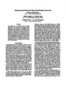
Figure 3: Formulas of type (2, 2, 3)-F((15, 15, 15), C). The x-axis is the ratio of clauses to 15, the number of existential variables in the innermost block X1 .
0.2
0 6
6.5
7
7.5
8
8.5
9
9.5
10
10.5
11
ratio=clauses/(existential variables)
Figure 2: Probability of truth of random (2, 3)-QBF formulas with 80 variables. Examining each value of ρ individually, we see that as the number of clauses is increased, the formulas change from being almost certainly true to almost certainly false. Moreover,
Figure 3 shows results on (2, 2, 3)-QBF formulas in which each quantifier block has 15 variables, for a total of 45 variables. When there is an odd number of quantifier blocks, a solver can conclude truth of a formula as soon as it finds an assignment to the outermost quantifier block such that the rest of the formula is true. Accordingly, for an odd number of quantifier blocks, the hardness drops down more slowly on the right of the peak (the “false” region) than on the left (the
“true” region). This slowness in dropping down on the right is quite pronounced in Figure 3. Note that a dual phenomenon takes place for an even number of quantifier blocks; see for example Figure 1. 1.2e+09
1 (3,3) (35,35) prob
6e+08
0.5
4e+08
2e+08
0 11
12
13
14
15
16
17
18
0 19
ratio=clauses/(existential variables)
Figure 4: Formulas of type (3, 3)-F((35, 35), C). Figure 4 shows results on (3, 3)-QBF formulas with ρ = 1, that is, with the same number of existential and universal variables, 35 each, for a total of 70 variables. Interestingly, although the number of variables is less than in Figure 1, the hardest formulas (of Figure 4) are considerably harder than those of Figure 1, emphasizing the importance of the first parameter of our model, the tuple giving, for each quantifier block, the number of literals per clause. Figure 5 shows results for (1, 4)-QBF formulas with 80 variables. We again see that differences in ρ can dramatically affect complexity.2 70000 rho 0.6 (1,4) rho 1.0 (1,4) 60000
50000
time (s)
In this section, we present a number of theoretical results which concern techniques for proving lower and upper bounds on the purported threshold in our model. In the random SAT model, theoretical work generally studies asymptotic properties of the model, in particular, properties that hold as the number of variables approaches infinity. In this section, we will similarly be concerned with asymptotic properties of our model, and we assume that in parameterizations (jl , kl , . . . , j1 , k1 )-F((ml , nl , . . . , m1 , n1 ), C)
8e+08 probability sat
number of branches
1e+09
3 Theoretical results
40000
30000
20000
10000
0 11
12
13
14
15
16
17
ratio=clauses/(existential variables)
Figure 5: Formulas of type (1, 4)-F((30, 50), C) and (1, 4)-F((40, 40), C).
and (kl , jl−1 , . . . , j1 , k1 )-F((nl , ml−1 , . . . , m1 , n1 ), C) of our model, the ki and ji are constant, but the ni , mi , and C are all functions of an underlying argument n. We will discuss properties that hold almost surely by which we mean with probability tending to one as n approaches infinity. Our first result concerns a way of obtaining threshold upper bounds, that is, “almost surely false” results. To illustrate the idea, let us focus on (j, k)-QBF formulas with two quantifier blocks, which are of the form ∀Y1 ∃X1 φ. Consider the game view (mentioned in the introduction) of such a formula: the universal player wishes to set Y1 so that the resulting formula cannot be satisfied by the existential player. A reasonable tactic for the universal player is to attempt to set the variables Y1 so that the number of clauses in the resulting formula is maximized. Suppose that the universal player chooses a setting to Y1 in such a way that she does not “look at” the existential literals of the formula–that is, the choice of assignment to Y1 depends only on the universal literals in the formula. With this form of choice, in a sense that can be made precise, the resulting formula (over X1 ) can be verified to be a random SAT formula. If the universal player can guarantee that the resulting random SAT formula has sufficiently many clauses, then almost sure falsity follows by making use of SAT threshold upper bounds. Let us be a bit more precise. We show how to obtain almost sure falsity results for formulas of the form (j, k)-F((m, n), D). Assume that k-F(n, C) formulas are almost surely false, that is, C/n is an upper bound for the k-SAT threshold. If we restrict such a formula to the universal literals (the Y1 literals), we obtain a j-F(m, D) formula. Assume further that D ≥ C is sufficiently high so that (almost surely) a j-F(m, D) has an assignment leaving C clauses unsatisfied. (In notation, we assume that minSAT(j-F(m, D)) ≤ D − C almost surely, where minSAT(F ) denotes the minimum, over all assignments, of the number of clauses satisfied in the formula F .) Together, these two assumptions, in light of the above discussion, imply that (j, k)-F((m, n), D) formulas are almost surely false. The following proposition is a formal statement of this claim, but in a more general form. Proposition 3.1. Suppose that instances of (kl , jl−1 , . . . , j1 , k1 )-F((nl , ml−1 , . . . , m1 , n1 ), C)
2
Note that in Figure 5, we use execution time instead of number of branches as a measure of hardness. This is because in some cases, the number of branches was so high that it was not correctly reported by the solver (in particular, overflow occurred).
are almost surely false, and that D is sufficiently high so that almost surely, it holds that minSAT(jp , kp , . . . , kl+1 , jl )-F((mp , np , . . . , nl+1 , ml ), D)
is less than or equal to D − C. Then, instances of (jp , kp , . . . , j1 , k1 )-F((mp , np , . . . , m1 , n1 ), D) are almost surely false. Note that one can formulate a dual of Proposition 3.1 that allows one to infer “almost surely true” results from previous “almost surely true” results, and that concerns maxSAT instead of minSAT. We next observe that, given a parameterization (of the model), if the parameterization is almost surely true after the elimination of a “prefix”, then the original parameterization is almost surely true. This permits, for instance, the derivation of “almost surely true” results for formulas beginning with a universal quantifier from such results for formulas beginning with an existential quantifier. Proposition 3.2. Let (jl , kl , . . . , j1 , k1 )-F((ml , nl , . . . , m1 , n1 ), C) be a parameterization of the model. If for some i < l it holds that instances of (ji , ki , . . . , j1 , k1 )-F((mi , ni , . . . , m1 , n1 ), C) or (ki+1 , ji , . . . , j1 , k1 )-F((ni+1 , mi , . . . , m1 , n1 ), C) are almost surely true, then instances of (jl , kl , . . . , j1 , k1 )-F((ml , nl , . . . , m1 , n1 ), C) are almost surely true. Proposition 3.2 follows from the general fact that a quantified formula Φ is true if eliminating one or more quantifier blocks from the outside of Φ, along with their associated literals, gives a true formula. Example 3.3. We demonstrate how to make use of the two propositions given so far by explicitly computing some threshold bounds for our model. We will consider (2, 3)-F((ρn, n), cn) formulas, that is, formulas of the type considered in Figures 1 and 2. We begin by looking at the case where ρ = 1, that is, (2, 3)-F((n, n), cn) formulas. We can use Proposition 3.1 specialized to two quantifier blocks (that is, with p = l = 1) to obtain an upper bound of c = 14.5 for such formulas, as discussed prior to the statement of that proposition. How is this done? The first requisite ingredient is a value cu such that 3-F(n, cu n) formulas are almost surely false, that is, a SAT threshold upper bound. By [Dubois et al., 2000], we can take cu = 4.506. The second ingredient needed is an upper bound for minSAT(2-F(n, cn)). By Theorem 3.5, which is presented below, we have that minSAT(2-F(n, cn)) ≤ (0.657)cn for c = 14.5. Using the proposition with C = cu n and D = 14.5n, we see that (0.657)cn ≤ (14.5n) − (cu n) and hence we have minSAT(2-F(n, cn)) ≤ D − C as required. Therefore, instances of (2, 3)-F((n, n), cn) are almost surely false for c = 14.5 (and hence for all c ≥ 14.5). Now let cl be a lower bound on the 3-SAT threshold, so that instances of 3-F(n, cl n) are almost surely true. We can take cl = 3.52 by [Kaporis et al., 2003]. By Proposition 3.2,
instances of (2, 3)-F((n, n), cl n) are almost surely true. The idea is that (2, 3)-F((n, n), cl n) formulas are almost surely true because after “eliminating” the first quantifier block in such formulas, one obtains 3-F(n, cl n) formulas, which are almost surely true by our choice of cl . To summarize the results observed so far, we have that (2, 3)-F((n, n), cn) instances are almost surely true when c ≤ cl = 3.52, and almost surely false when c ≥ 14.5. Now, let us consider (2, 3)-F((ρn, n), cn) formulas. Regarding lower bounds, as before, we have by Proposition 3.2 that instances of (2, 3)-F((ρn, n), cl n) are almost surely true. Turning to upper bounds, we observe that, by a standard probabilistic argument, every 2-SAT formula has an assignment satisfying (at most) 3/4 of the clauses. Thus, we have minSAT(2-F(ρn, 4cu n)) ≤ 3cu n for any value of ρ. Using Proposition 3.1 as before with C = cu n and D = 4cu n, we obtain that instances of (2, 3)-F((ρn, n), cn) are almost surely false for c ≥ 4cu , that is, 4cu is a threshold upper bound on formulas (2, 3)-F((ρn, n), cn), for any value of ρ. Summarizing, we have obtained that for any value of ρ, formulas (2, 3)-F((ρn, n), cn) are almost surely false when c ≤ cl , and almost surely true when c ≥ 4cu . That is, such formulas change from being almost surely true to almost surely false between cl and 4cu . If we set cl and cu to 4.26, which is an approximate value of the 3-SAT threshold, we expect the threshold for such formulas to lie between c = 4.26 and c = 4 · 4.26 = 17.04, where c denotes the ratio of clauses to existential variables; this expectation is consistent with Figure 2. In the usual random SAT model, whenever the clause length is fixed, it is known that at a sufficiently low constant clause-to-variable ratio, formulas are almost surely satisfiable, and that at a sufficiently high constant clause-to-variable ratio, formulas are almost surely unsatisfiable. These results, of course, validate the hypothesis that there is a threshold phenomenon in this model. We can show analogous results in our model. Proposition 3.4. Fix (jl , kl , . . . , j1 , k1 ) to be a tuple with k1 ≥ 2, and for i ∈ {1, . . . , l}, let ni (n) be a linear function of n, that is, ni (n) = σi n for a constant σi > 0. There exist positive constants al and au such that instances of (jl , kl , . . . , j1 , k1 )-F((ml , nl , . . . , m1 , n1 ), cn) are almost surely true when c ≤ al , and instances of (jl , kl , . . . , j1 , k1 )-F((ml , nl , . . . , m1 , n1 ), cn) are almost surely false when c ≥ au . (This proposition is meant to address formulas with both even and odd numbers of quantifier blocks, that is, we permit jl = 0.) The “almost surely true” part follows from Proposition 3.2 along with known lower bounds on the SAT threshold, while the “almost surely false” part follows from the fact that shifting existential quantifiers inward preserves truth of quantified formulas, the idea of Proposition 3.1, and a standard first moment argument. We now study threshold upper bounds for our model in greater detail. Proposition 3.1 establishes a connection between minSAT and upper bounds in our model. Although
minSAT has not, as far as we know, been studied explicitly in previous work, we certainly believe that it is a natural concept of independent interest. We have the following result concerning it. Theorem 3.5. For every k ≥ 2, there exists a function gk such that for all c > 0, it holds almost surely that minSAT(k-F(n, cn)) ≤ gk (c)cn + o(n). We plot obtainable g2 and g3 in Figure 6, comparing them against the values 3/4 and 7/8 obtainable by a standard probabilistic argument. We prove this theorem by analyzing a simple algorithm similar to one used in the paper [Coppersmith et al., 2003] to study maxSAT. The algorithm is analyzed using the differential equation approach of [Wormald, 1995] that has been used in many random SAT threshold lower bound arguments. 0.9
upper bound minSAT
0.8 0.75 0.7 0.65 0.6 0.55 0.5 0.45 0
2
4
6
8
10
12
14
16
18
Acknowledgements. The authors wish to thank V´ıctor Dalmau and Bart Selman for helpful comments, and Massimo Narizzano for his help with QuBE.
References
2-SAT expected 2-SAT 3-SAT expected 3-SAT
0.85
Theorem 3.7. For all constants k ≥ 2 and c > 0, there exists a constant x > 0 depending on k and c such that all size xcn subformulas of k-F(n, cn) are satisfiable almost surely. The proof of Theorem 3.7 makes use of [Chvatal and Szemeredi, 1988, Lemma 1]. Proposition 3.6 and Theorem 3.7 can be used together to obtain threshold lower bounds for ∀∃ formulas. In particular, notice that in Proposition 3.6, relative to fixed c and ρ, increasing j allows one to decrease x. Moreover, the lower the x required in Theorem 3.7, the higher the c may be. Thus, fixing k and ρ, increasing j allows us to obtain higher and higher lower bounds on the threshold of (j, k)-F((ρn, n), cn).
20
22
ratio=clauses/(variables)
Figure 6: Upper bounds for minSAT(k-F(n, cn)) from Theorem 3.5. Now we look further at threshold lower bounds in our model, focusing on formulas with quantifier prefix ∀∃. One can observe that if all “small” subformulas of a random SAT formula are satisfiable, at clause-to-variable ratio c, then formulas at clause-to-variable ratio c are true. Proposition 3.6. Fix a tuple (j, k) and constants c, ρ > 0. There exists a positive constant x < 1 (depending on j, c, and ρ) such that if all subformulas of size xcn in an instance of k-F(n, cn) are satisfiable almost surely, then instances of (j, k)-F((ρn, n), cn) are true almost surely. Proposition 3.6 follows from the fact that a sufficiently small y > 0 can be picked so that the probability of minSAT(j-F(ρn, cn)) ≤ ycn converges to zero. This can be proved by using a union bound and Chernoff bounds on a first moment. The desired x can then be obtained as (1 − y). This “small subformula” property has not been previously studied to our knowledge, but as with minSAT, we believe that it is a natural concept of possible independent interest. We can show that this property holds for random SAT formulas, for subformulas having size equal to a constant fraction of the number of clauses.
[Cadoli et al., 1999] Marco Cadoli, Marco Schaerf, Andrea Giovanardi, and Massimo Giovanardi. An algorithm to evaluate quantified boolean formulae and its experimental evaluation. Technical report, Dipartimento di Informatica e Sistemistica, Universita di Roma ”La Sapienza”, 1999. [Chvatal and Szemeredi, 1988] V. Chvatal and E. Szemeredi. Many hard examples for resolution. Journal of the Association for Computing Machinery, 35:759–768, 1988. [Coppersmith et al., 2003] D. Coppersmith, D. Gamarnik, M. Hajiaghayi, and G. Sorkin. Random max 2-sat and max cut, 2003. [Dubois et al., 2000] Olivier Dubois, Yacine Boufkhad, and Jacques Mandler. Typical random 3-sat formulae and the satisfiability threshold. In SODA, pages 126–127, 2000. Full version in Electronic Colloquium on Computational Complexity (ECCC 2003). [Gent and Walsh, 1999] Ian P. Gent and Toby Walsh. Beyond NP: the QSAT phase transition. Proceedings of AAAI 1999, 1999. [Giunchiglia et al., 2001] Enrico Giunchiglia, Massimo Narizzano, and Armando Tacchella. QUBE: A system for deciding quantified boolean formulas satisfiability. Proceedings of the International Joint Conference on Automated Reasoning, 2001. [Kaporis et al., 2003] Alexis C. Kaporis, Lefteris M. Kirousis, and Efthimios Lalas. Selecting complementary pairs of literals. Electronic Notes in Discrete Mathematics, 16, 2003. [Mitchell et al., 1992] D. Mitchell, B. Selman, and H. Levesque. Hard and easy distributions of sat problems. In Proc. 10-th National Conf. on Artificial Intelligence, pages 459–465, 1992. [Wormald, 1995] N. C. Wormald. Differential equations for random processes and random graphs. Annals of Applied Probability, 5(4):1217–1235, 1995.