382
IEEE TRANSACTIONS ON ROBOTICS AND AUTOMATION, VOL. 16, NO. 4, AUGUST 2000
First-Order Hybrid Petri Nets: A Model for Optimization and Control Fabio Balduzzi, Member, IEEE, Alessandro Giua, and Giuseppe Menga
Abstract—We consider in this paper first-order hybrid Petri Nets, a model that consists of continuous places holding fluid, discrete places containing a nonnegative integer number of tokens, and transitions, either discrete or continuous. We set up a linear algebraic formalism to study the first-order continuous behavior of this model and show how its control can be framed as a conflict resolution policy that aims at optimizing a given objective function. The use of linear algebra leads to sensitivity analysis that allows one to study of how changes in the structure of the model influence the optimal behavior. As an example of application, we show how the proposed formalism can be applied to flexible manufacturing systems with arbitrary layout and different classes of products. Index Terms—Flexible manufacturing systems, hybrid Petri nets, optimization, performance evaluation, sensitivity analysis.
I. INTRODUCTION A. Motivation
T
HE CONTROL of hybrid systems, i.e., systems with both continuous-time and discrete-event dynamics, is a domain of increasing importance and several hybrid models have been presented in the literature. Petri nets (PN’s) [17] have originally been introduced to describe and analyze discrete event systems. Recently, much effort has been devoted to apply these models to hybrid systems (see Section I-C for a discussion of relevant literature). The usual tradeoff between modeling power and analytical tractability also applies to hybrid PN models. On one hand, there exist Markovian models with a powerful set of analytical tools [22]. On the other, there exist models that can describe larger classes of systems but that can be validated only by simulation [10], or possibly if the incidence matrix can be defined for them, by invariant analysis [2], [3], [14], [16]. In this paper, we present a model called first-order hybrid PN’s (FOHPN’s) [6]–[8] that is general enough to model classes of systems of practical interest and yet whose first-order continuous behavior can be studied by linear algebraic tools. An FOHPN consists of continuous places holding fluid, discrete places containing a nonnegative integer number of tokens and Manuscript received September 22, 1998; revised August 23, 1999. This paper was recommended for publication by Associate Editor M. Zhou and Editor P. Luh upon evaluation of the reviewers’ comments. This paper was presented in part at the IEEE International Conference on Systems, Man and Cybernetics, San Francisco, CA, Ocotober 1998, and in part at the 4th Workshop on Discrete Event Dynamics Systems, Calgiari, Italy, August 1998. F. Balduzzi and G. Menga are with the Dipartimento di Automatica e Informatica, Politecnico di Torino, Torino, Italy (e-mail:
[email protected];
[email protected]). A. Giua is with the Dipartimento di Ingegneria Elettrica ed Elettronica, Università di Cagliari, Cagliari, Italy (e-mail:
[email protected]). Publisher Item Identifier S 1042-296X(00)06959-7.
transitions, either discrete or continuous. We assume that an autonomous timing structure (deterministic or stochastic) is associated to the discrete transitions. On the contrary, we assume that the instantaneous firing speeds (IFS) of the continuous transitions are control variables which may be chosen by the system , where is the number operator within a given set . of continuous transitions and In the paper, we address two main issues: on-line control and structural optimization. The on-line control problem, i.e., the , corresponds to a computation of an optimal IFS vector conflict resolution. Conflict resolution is an important issue in the study of discrete nets. Conflicts arise when a limited number of tokens enables more than one transition, but it is only sufficient to fire a subset of them. Several schemes have been devised to tackle this problem for discrete timed nets, including token reservations [2], resampling rules, and priorities [1]. To any of these schemes corresponds a timing structure which imposes an a priori scheduling policy, i.e., the firing of discrete transitions is not controlled on-line. In FOHPN’s, we adopt a similar approach and we assume that discrete transitions fire according to their timing structure. Note that this is not a limitation, as these transitions are generally used to represent the occurrence of events whose delay is not controllable (e.g., the failure or the repair of a machine). The on-line control problem we address in this paper is that of computing an “optimal” mode of operation of the net by solving conflicts among continuous transitions at continuous places where continuous flows must be routed in the net. The choice of an optimal IFS vector is framed as a linear programming problem (LPP). This leads quite naturally to the structural optimization problem. In fact, the use of linear programming and sensitivity analysis tools allows one to study of how changes in the structure of the model influence the optimal behavior. In the final section, we discuss as an example of application a manufacturing system. Manufacturing systems are discrete event systems whose number of reachable states is typically very large, hence approximating fluid models have often been used in this context [5], [11], [21]. The FOHPN model is rich enough to model manufacturing systems consisting of unreliable machines and buffers of finite capacity in the most general multiclass multimachine setting. Several criteria to assess performances of a manufacturing system, such as throughput rate, buffer levels, machines utilization, etc., can be framed as conflict resolution policies for the FOHPN model. In addition, a designer or analyst of a manufacturing system may want to perform “what if” analysis. For example, what happens to throughput if a machine produces faster? These problems
1042–296X/00$10.00 © 2000 IEEE
BALDUZZI et al.: FIRST-ORDER HYBRID PN’S: A MODEL FOR OPTIMIZATION AND CONTROL
will be addressed applying sensitivity analysis to the FOHPN model.
383
changes in the structure of the model influence its optimal behavior. C. Relevant Literature
B. Proposed Model In the first part of the paper, we describe a general hybrid PN model based on the framework proposed by Alla and David [2]. As in all hybrid models, we distinguish two behavioral levels. At the lower level, the continuous evolution of the net is described by first-order fluid models, i.e., models in which the continuous flows have constant rates and the fluid content of each continuous place varies linearly with time. Each model is relative to a given macrostate characterized by the following: 1) the discrete marking of the net and 2) the set of empty continuous places. The macro-state defines the set of admissible IFS vectors of continuous transitions. Since we consider the first-order behavior, we assume that the IFS vector remains constant within a macro-state. At the higher level, a discrete-event model describes the macro-behavior of the net that, upon the occurrence of macro-events, evolves through a sequence of macro-states. As it will be clear in the formal description of the model, we consider the following two types of macro-events: 1) the firing of a discrete transition, according to a given timing structure, and 2) the emptying of a continuous place. A useful formalism for the analysis of discrete timed nets, assumes that the timing structure associated to the transitions is stochastic with exponentially distributed delays (see, e.g., [1]). This has the advantages of leading to a Markovian model that can be easily analyzed. In our model, however, the occurrence of the second type of macro-events does not preserve the Markovian property, hence, we allow arbitrary stochastic or deterministic timing structures. Thus, the resulting macro-behavior can be described as a generalized semi-Markovian process (GSMP). The key features that represent the novelty of our approach are the following. • We allow the IFS of a continuous transition to be chosen , where is by a control agent in a given range is the maximum the minimum firing speed (mfs) and firing speed (MFS). • We explicitly define the set of all admissible IFS vectors within a given macro-state. This set is characterized by the feasible solutions of a linear constraint set. • We consider the problem of choosing an optimal IFS vector according to a given objective function. Our optimization scheme can only be myopic [5], in the sense that it generates a piecewise optimal solution, i.e., a solution that is optimal only in a macro-state. Although we provide the basic tools for the analysis of the overall behavior of a net, this paper is only concerned with the analysis and optimization within a macro-state. • We adopt the optimal basis approach, i.e., the simplex method, to solve LPP. We show how one can naturally apply to the FOHPN framework those sensitivity analysis techniques that pertain to LPP [15], [19] to study how
The hybrid PN model we propose follows the formalism described by David and Alla [2], [3]. In effect, our model can be seen as an extension of timed hybrid nets with constant maximal speeds with the following additional features: token reservation is not used as a conflict resolution policy; stochastic transitions are also included in our model; minimal firing speeds are considered as well. The novel contribution of our work is that of showing how the first-order behavior of such a net can be efficiently analyzed with a linear algebraic formalism. Linear algebraic techniques have also been used by Amrah et al. [4] when modeling manufacturing systems with continuous PN’s. These authors deal with open and closed transfer lines modeled by controlled variable speed continuous PN’s, a type of continuous PN [3] with controllable maximal firing speeds. Then by using a constrained optimization approach, they obtained optimal values for the machine production rates that bring the average levels of buffers to a desired values. However, it must be observed that transfer lines are not a general model, in the sense they do not require scheduling and routing. Our work, instead may deal with manufacturing systems in the more general configurations and settings. Another approach that extends the stochastic discrete PN framework of [1] toward fluid approximations is fluid stochastic PN’s presented by Trivedi and Kulkarni [22]. These authors proposed a model with places holding continuous tokens and arcs representing fluid flows. The flow rates are uniquely specified by the complete marking of the net. This is a main difference with our approach, in which the IFS vector of continuous transitions can be chosen in a given set that defines all admissible ones. All these hybrid models discussed so far are fluid models, i.e., the marking of the continuous places is a nonnegative real number. However, more general hybrid PN’s that also admit negative-real markings have been proposed. Differential PN’s have been presented by Demongodin and Koussoulas [14] and can be used to model hybrid systems whose continuous evolution can be described by a finite number of linear first-order differential state equations. High-level hybrid PN’s [16] extend the hybrid framework to colored nets: the use of real numbers as colors allows one to model general primitives such as jumps in the state space and switches in the continuous dynamics, which cannot be generally described with other formalisms. In other approaches [10], the PN formalism is only used to represent the discrete state of a hybrid system, while the continuous state is represented by a vector (not by a marking) whose arbitrary continuous evolution is modeled by differential algebraic equations. The rest of the paper is structured as follows. In Section II, we introduce FOHPN’s. Section III is concerned with the computation of the instantaneous firing speed of continuous transitions and with different conflict resolution schemes. Section IV deals with the sensitivity analysis of this model. In Section V, we apply the previously developed results to a manufacturing system.
384
IEEE TRANSACTIONS ON ROBOTICS AND AUTOMATION, VOL. 16, NO. 4, AUGUST 2000
II. BACKGROUND We recall the PN formalism used in this paper. For a more comprehensive introduction to place/transition PN’s, see [17]. The common notation and semantics for timed nets can be found in [1]. Hybrid PN’s are defined in [2]. Fig. 1. FOHPN.
A. Structure and Marking . An FOHPN is a structure is partitioned into a set of disThe set of places (represented as circles) and a set of continuous crete places (represented as double circles). places is partitioned into a set The set of transitions and a set of continuous transitions of discrete transitions (represented as double boxes). The set is (reprefurther partitioned into a set of immediate transitions (repsented as bars), a set of deterministic timed transitions resented as black boxes), and a set of exponentially distributed (represented as white boxes). The carditimed transitions is denoted , , and . nality of , , and The pre- and post-incidence functions that specify the arcs are1
and
We require (well-formed nets) that for all and for all , . specifies the timing associThe function ated to timed discrete transitions. We associate to a deterministic its (constant) firing delay . timed transition We associate to an exponentially distributed timed transition its average firing rate , i.e., the average firing , where is the parameter of the corresponding delay is exponential distribution. specifies the firing speeds The function : associated to continuous transitions.2 For any continuous tran, we let , with . Here sition represents the mfs and represents the MFS. In the following, unless explicitly specified, the mfs of a continuous transition . will be We denote the preset (postset) of transition as ( ) and its restriction to continuous or discrete places as or . Similar notation may be used for presets and postsets of places. The incidence matrix of the net is defined . The restriction of to as and ( ) is denoted . Note that by the . well-formed hypothesis, A marking (1) is a function that assigns to each discrete place a nonnegative number of tokens, represented by black dots and assigns to each 1Here 2Here
= =
[ f0g. [ f1g.
continuous place a fluid volume; denotes the marking of . place . The value of a marking at time is denoted and are denoted with and , The restriction of to respectively. is an FOHPN with an iniAn FOHPN system . tial marking B. Enabling and Firing The enabling of a discrete transition depends on the marking of all its input places, both discrete and continuous. be an FOHPN system. A discrete Definition 1: Let , . transition is enabled at if for all An enabled discrete transition fires (after its associated . The firing of delay) yielding the marking discrete transitions may follow any of the common enabling and firing rules discussed in [1]. These rules—that define the structure of the GSMP associated to the net—are well known and are not further discussed in this paper. A continuous transition is enabled only by the marking of its input discrete places. The marking of its input continuous places, however, is used to distinguish between strongly and weakly enabling. be an FOHPN system. A continDefinition 2: Let if for all , uous transition is enabled at . is: We say that an enabled transition , ; • strongly enabled at if for all places , . • weakly enabled at if for some Remark 3: We note that the definition of enabling we have given is slightly different from the one proposed by David and Alla in [3], where it was also required that a weakly enabled transition be “fed,” i.e., that there exists an upstream transition strongly enabled feeding it. The two notions lead to different semantics for a cycle such as the one in Fig. 1. According to the definition of [3], the two transitions are not enabled and the cycle is blocked, while according to our definition they are both weakly enabled and the cycle is not blocked. To overcome this limitation, David and Alla introduced in [13] a new concept—that of -marking. If an arbitrary small marking is initially assigned to any of the two places of the cycle in Fig. 1, then both transitions can be considered weakly enabled. Thus, in this generalized framework, it is possible to assign to empty cycles two semantics: blocked cycles (those that are empty) and nonblocked cycles (those -marked). We believe that blocked cycles are not a useful modeling feature for systems of practical interest, thus we have chosen to keep just the second semantics. The enabling state of a continuous transition defines its admissible instantaneous firing speed (IFS) .
BALDUZZI et al.: FIRST-ORDER HYBRID PN’S: A MODEL FOR OPTIMIZATION AND CONTROL
Fig. 2.
385
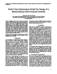
(a) An FOHPN, (b) its phase-diagram, and (c) its evolution in time.
Definition 4: Let be an FOHPN system and be a continuous transition with IFS . . • If is not enabled, then • If is strongly enabled, then it may fire with any firing . speed • If is weakly enabled, then it may fire with any firing , where depends on the speed amount of fluid entering the empty input continuous place(s) of . In fact, the transition cannot remove more fluid from any empty input continuous place than the quantity entered in by other transitions. The computation of the IFS of enabled transitions is not a trivial task. We will set up in Section III a linear-algebraic formalism to do this. Here, we simply discuss the net evolution assuming that the IFS are given. is denoted . The The IFS at time of a transition is described evolution in time of the marking of a place by (2) Indeed. (2) holds assuming that at time no discrete transition are continuous in . is fired and that all speeds
length . Let be the firing count vector at time , i.e., that specifies the discrete transitions, a vector of dimension if any, firing at time . Thus, the micro-behavior of an FOHPN is described during the th macro-period by (3) , while the evolution of the net at the ocwhere currence of the macro-events is described by (4) The macro-behavior of an FOHPN can be described by a phase-diagram in which every macro-state is represented by a of the corresponding box labeled on the right by the length macro-period. Each box is partitioned into two parts. On the left of the net is represented. (discrete part) the discrete marking of the On the right (continuous part) the continuous marking net at time is represented with the IFS vector . Macro-states are connected through bars, representing the macro-events that caused the state transitions. Each bar is labeled on the left (respectively, right) by the discrete transition (respectively, continuous place) that caused the occurrence of the macro-event. An example is discussed in the following section.
C. Net Dynamics
D. Example
A macro-event occurs when: 1) either a discrete transition fires, thus changing the discrete marking or enabling/disabling a continuous transition or 2) or a continuous place becomes empty, thus changing the enabling state of a continuous transition from strong to weak. and be the occurrence times of consecuLet is called tive macro-events; the interval of time . macro-period and its length is denoted We will assume that the IFS of continuous transitions are constant during a macro-period. Thus, the discrete marking and the IFS vector during a macro-period define a macro-state that corresponds to the invariant behavior states of [2]. We now describe the dynamics of an FOHPN. Let be the be the instants in which macro-events initial time, be the IFS vector during the macro-period of occur, and
Consider the net in Fig. 2(a) and let the initial time be . is a continuous place with initial marking Place . Places , , , are discrete places. Transitions and are continuous transitions with MFS and . We as(here and are the arc weights given by sume and ). Discrete transitions , , , are exponentially distributed timed transitions whose average firing rates are , , , and , respectively. Macro-Period MP0: In the initial state, is not empty and , are marked. Thus, transitions and are strongly enabled and may fire at their maximum speeds, i.e., we choose and . The continuous marking of the net during this macro-period is given, as in (2), by
386
Fig. 3.
IEEE TRANSACTIONS ON ROBOTICS AND AUTOMATION, VOL. 16, NO. 4, AUGUST 2000
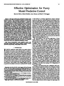
FOHPN model of (a) a conflict-free re-entrant production line, (b) a free-choice conflict, and (c) a non free-choice conflict.
while the discrete marking is constant and given by
Macro-Period MP1: At time , place becomes empty, thus causing a macro-event. In the new macro-state, remains strongly enabled, while is weakly en. Asabled and may fire at most at speed and . Then, the continuous marking sume . of the net during this macro-period is constant: The discrete marking maintains the value it had in the previous macro-period since no discrete transition has fired. Macro-Period MP2: We assume that the enabled transition fires at time . This macro-event changes the discrete . Now transition marking of the net to is disabled, i.e., , while remains strongly enabled. . Then, the continuous marking during this Assume macro-period is given, as in (2), by
This behavior is represented in Fig. 2(b) and (c), which shows , the phase-diagram of this net and the evolution in time of , .
to a particular objective function. Note that each set corresponds to a particular system macro-state. Thus, our optimization scheme can only be myopic [5], in the sense that it generates a piecewise optimal solution, i.e., a solution that is optimal only in a macro-period. • We compute a particular (optimal) IFS vector solving a linear programming problem, rather than by means of an iterative algorithm, whose convergence properties may not be good. • Linear programming leads to sensitivity analysis, which plays an essential role in performance evaluation and optimization. In fact, we may be able to compute analytically the objective function improvement due to a parameter variation. A. Admissible IFS Vectors In this section, we characterize the set of admissible IFS vectors. be an FOHPN system with conDefinition 5: Let tinuous transitions and incidence matrix . Let ( ) be the subset of continuous transitions enabled be the (not enabled) at , and subset of empty continuous places. Any admissible IFS vector at is a feasible solution of the following linear set:
III. FIRING SPEED AND DYNAMICS OF AN FOHPN The computation of an admissible IFS vector of continuous and hybrid nets is not trivial. In [3], an iterative algorithm was given to determine a single admissible vector; the algorithm aims at maximizing firing speeds while respecting priority rules. We propose a different approach in which we use linear inequalof all admissible firing ities to characterize the set represents a particular mode speed vectors. Each vector of operation of the system described by the net, and among all possible modes of operation, the system operator may choose the best according to a given objective. There are several advantages in our approach. • We can explicitly characterize the set of all admissible IFS vectors in a given macro-state and not just compute a particular vector. • We consider more general scheduling rules than priorities. For example, in an FMS, we may want to maximize machines utilization, maximize the throughput of the system, balance the load, etc. Each of these problems corresponds
(5)
. The set of all feasible solutions is denoted Thus, the total number of constraints that define is: card card card (here, denotes the cardinality of the set ). Constraints of card the form (5.a)–(5.c) follow from the firing rules of continuous transitions. Constraints of the form (5.d) follow from (2), because if a continuous place is empty then its fluid content cannot decrease. , then the constraint of the form (5.b) Note that if associated to reduces to a nonnegativity constraint on . be the net in Fig. 3(a), with Example 6: Let , where place is initially empty. Such a net is represen-
BALDUZZI et al.: FIRST-ORDER HYBRID PN’S: A MODEL FOR OPTIMIZATION AND CONTROL
tative of a re-entrant production line. Hence, according to the previous definition
(6)
. is the linear constraint set that defines We now discuss under which conditions the set admits feasible solutions. When no feasible solution exists, no admissible modes of operation is allowed by the net. First, we make the following observation. Remark 7: Any constraint of the form (5d) related to an empty continuous place can be written as (7) and . The set (respectively, ) with contains the indices of the continuous transitions whose firing increases (respectively, decreases) the marking of . Definition 8: Let be an FOHPN system. A transition is called mfs-free at if at least one of the following conditions holds: ; 1) the mfs of is has no empty input continuous places, i.e., 2) . We can now provide a sufficient condition for the existence of admissible IFS vectors. be the linear set defined by (5). Proposition 9: Let are mfs-free at . Such a set is nonempty if all be such that if , Proof: Let . We prove that . else Clearly this vector satisfies all constraints of the form (5a)–(5c). Moreover, from Remark 7, it follows that any constraint of the form (5d) can be written as
and the right-hand side of this equation evaluates to 0 by the assumption that all enabled transitions are mfs-free. Thus, this constraint is satisfied. As a counterexample, we show that no feasible solution may exist if one (or more) continuous transition is not mfs-free. . Let Example 10: Consider the net in Fig. 3(a) with and . Thus, transition is not is defined by the following set of mfs-free. The set inequalities:
uous places, since the computation of an admissible IFS vector is only affected by this type of conflicts. Example 11: Consider the net shown in Fig. 3(b). When place is not empty, both and can fire at their MFS. When is bounded place is empty, however, the output flow there will be a constraint by the input flow , thus in . This of the form (5d) related to place that writes constraint expresses the fact that we have a limited amount of resource (the input flow) that must be shared between different processes (the output transitions). There is no conflict in a net, instead, if each empty place has at most one enabled output transition . This motivates the next definition. be an FOHPN system and Definition 12: Let be the linear set defined by (5). We say that is continuous conflict-free (CCF) at if for all constraints of the . form (5d) rewritten as (7) holds: card In the rest of this section, we discuss the relationship between conflict resolution (i.e., the computation of IFS vectors) and performance optimization. If we set our goal to maximize the firing speed of the continuous transitions, it is possible to show that in a continuous conflict-free FOHPN each component of the IFS vector may be maximized independently. be an FOHPN system. If is CCF Theorem 13: Let of the following LPP at , the optimal solution s.t.
is such that Proof: Let
, (componentwise). be the (componentwise) operator, i.e., . It is sufficient to prove that if the net is CCF, then . will satisfy all Clearly, if and satisfy (5), then constraints of the form (5a)–(5c). Under the hypothesis of conflict-freeness, we can write any constraint of the form (5d) associated to a place as follows: if no enabled transition outputs from 1) place ; if is the only enabled tran2) sition outputting from place ; , , . with , In the first case, we have that
(8) while in the second case, we have that clearly admits no feasible solution. B. Conflict-Free Firing Speed Computation By the formalism previously introduced, we define the concept of conflict in a net. We will only treat conflicts at contin-
387
388
IEEE TRANSACTIONS ON ROBOTICS AND AUTOMATION, VOL. 16, NO. 4, AUGUST 2000
i.e., the vector satisfies all constraints of the form (5d) as well. In the case of CCF nets, the optimal solution in the previous theorem coincides with the solution computed with the priority algorithm in [3]. It may be interesting, however, to compare the two algorithms via an example. Example 14: Let us consider again the net in Fig. 3(a) whose set of admissible IFS vectors is given by (6). If we compute solution of (6) that maximizes , we the vector and . This clearly obtain example is so simple that we can write the solution in closed form; in more complex cases, the solution can still be easily found solving the associated LPP. If we apply the procedure , proposed in [3], we obtain at the first iteration step while to compute the IFS of transition we need to solve the following iterative problem:
and for , the algorithm requires an infinite number of steps to converge to the correct value . C. Global Conflict Resolution When the net is not conflict-free, not all firing speeds may be maximized independently. However, we can always find out a conflict resolution policy by solving an LPP aimed at a global optimization of the system resources. We may consider different performance indices as the objective function in the LP formulation of the problem. We consider some examples. Maximize Flows: In an FOHPN, we may consider as optimal the solution of (5) that maximizes the performance index , which is of course intended to maximize the sum over all flow rates. In the manufacturing domain, this may correspond to maximizing machines utilization. Maximize Outflows: In an FOHPN, we may want to maxiwhere mize the performance index if if
is an exogenous transition, is an endogenous transition.
In the manufacturing domain, this may correspond to maximizing throughput. Dynamic Flow Balancing: This problem consists in reducing the difference between maximum and minimum utilization of continuous transitions. The utilization of can be given as the ratio . a transition Then, we may want to minimize the performance index for a suitable index set . In the manufacturing domain, this may correspond to balancing the machines load. Minimize Stored Fluid: In an FOHPN, we may want to min. This can imize the derivative of the marking of a place where be done by minimizing the performance index if otherwise.
,
In the manufacturing domain, this may correspond to minimizing the work-in-process (WIP). A different optimization procedure is based on global priorities (GP). In this case, we have a multiobjective performance in which the goals have different priorities. We first look for all solutions that optimize the first goal, then among them for those that optimize the second goal, and so forth. We discuss a simple case in which each goal consists in maximizing the IFS of a single transition, though this result can be easily generalized. Definition 15: Let be an FOHPN system and be the linear set defined by (5). Assume that the continuous transitions of the net are ordered in a priority . The GP-optimal solution for sequence is defined by
where . The GP-optimal solution can be found by solving LPP. First, we compute ; then, we add to (5) the constraint and maximize , etc. Note, however, that there exist other techniques based on lexicographic ordering [9] that may well be meaningfully used to compute the GP-optimal solution by solving a single LPP with a suitably modified objective function. Example 16: Consider the net in Fig. 3(c) with , , and places , initially empty. We apply the method discussed above to obtain . Note that by applying the algorithm , which is an proposed in [3], we obtain admissible IFS vector even though it does not have the same properties of the GP-optimal solution. According to the next theorem, a GP-optimal solution is , hence, it is a basic solution of any LPP subject to amenable to sensitivity analysis as it will be discussed in the following section. Theorem 17: The GP-optimal solution is unique and it is . a vertex, i.e., a basic solution, of the feasible region and Proof: Let for . We are also vertices of will prove that all vertices of . In fact, the hyperplane does not cut in any internal point because by the convex set . The solution construction is necessarily unique because for all if for and then cannot be a GP-optimal solution. D. Local Conflict Resolution The use of a performance index to be maximized (or minimized) over the space of all admissible IFS vectors corresponds to a global optimization procedure. It is often the case, however, that local rules are used to determine the operating mode of a system described by a hybrid net. These rules correspond to decisions that can be taken in a decentralized way.
BALDUZZI et al.: FIRST-ORDER HYBRID PN’S: A MODEL FOR OPTIMIZATION AND CONTROL
We consider the case of nets where all conflicts are freechoice, i.e., if a continuous place has more than one output with ), continuous transition (e.g., then it is the only continuous input place for all those transitions ). The conflict in Fig. 3(b) is (i.e., free-choice, while the two conflicts in Fig. 3(c) are not. When the conflicts are not free-choice, the local optimization rules described below may not be well founded. Fixed Ratio: One particular simple rule that may be used to locally solve free-choice conflicts is that of assigning a fixed ratio of fluid volume to all enabled continuous transitions that take fluid out of an empty continuous place. As an example, in , . This new Fig. 3(b), we may assign a ratio constraint can be added to the set or, even better, by substitution we can reduce by one the number of variables in (5). Local Priorities: We can also consider the case of local priority rules by a suitable modification of the linear set (5). Assume that in Fig. 3(b) a legal solution is such that has priority over , i.e., all fluid entering place should be consumed by and only if the remaining fluid should be consumed by . This can be done adding the following constraints:
where , with . Thus, if it . The problem with this technique is that a simple follows LPP is transformed into a more complex mixed integer-linear problem.
389
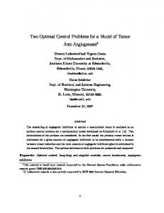
Fig. 4. (a) FOHPN model of a manufacturing service. (b) The feasible region for the IFS vectors.
Note that when , the slack and the corresponding constraint can be removed from the LPP given by (9) . by adding a nonnegativity constraint on variables, is the Here is a vector with matrix constraints, and we assume that has full rank, is the )-vector of the objective coefficients, while represents ( the -vector of the right-hand side constants. In this work, the simplex method will be used to solve LPP. This is an iterative method in which at each step and in an efficient manner, a new basis is computed. Each basis represents a vertex of the feasible region. We denote an optimal solution , the corresponding optimal basis (a set of variables), and the optimal basis matrix obtained by taking only those columns of whose corresponding variables are in . An optimal solucan always be written as tion
IV. SENSITIVITY ANALYSIS FOR FOHPN The LPP stated in the previous section may be solved taking into account only the constraints related to enabled transitions since we know that the IFS of transitions that are not enabled are be the set of indices of the enabled 0. Let be the set of continuous transitions and indices of the empty continuous places. Thus, we can write s.t.
The variables in are the basic variables, while the others, whose set is denoted , are called nonbasic. Note that the optimal solution may be degenerate, i.e., we have many basis associated with it. It may also be the case that more than one basic optimal solution exists. Example 18: In Fig. 4(a), it is represented the FOHPN model of a manufacturing service, where transition models an unand represent the outreliable machine and transitions flows from buffer . A buffer capacity 0 is imposed by the co-buffer place . The maximum production rate of the machine is bounded by the MFS , while the maximum outflows and , respectively. The discrete part rates cannot exceed of the net models the failure/repair stochastic process of the machine by means of exponential transitions and with average and , respectively. The machine is operating firing rates while place is marked (i.e., transition is enabled) and it is is marked. down when place The constraint set associated to this net from the given marking is
(9) Defining vector following standard form:
, we obtain the (11) (10)
390
IEEE TRANSACTIONS ON ROBOTICS AND AUTOMATION, VOL. 16, NO. 4, AUGUST 2000
We take as objective function to be maximized , representing the overall output flow, and we obtain the following LPP in standard form: s.t.
Note that we have not written the nonnegativity constraints and we have packed together the last two inequalities of (11). , There are infinitely many optimal solutions of the form , with , represented by the thick . Two of these are basic line in Fig. 4(b) in the plane and . Point solutions: is a nondegenerate solution with basic variables , , , and basis . Point is a degenerate and solution with two optimal basis: . Furthermore, we observe that in there is also another basis , which is not optimal. Sensitivity analysis refers to the study of how optimal solutions change according to changes of the given linear program in terms of the coefficients of the matrix, the right-hand side and the objective function. Suppose that the LPP (10) has an optimal solution. If there is any change in the values of , , or , the optimal solution is likely to change in general. In the next sections, we will develop sensitivity analysis with respect to the design parameters by assuming changes in the right-hand side vector and in the matrix coefficients. Perturbations in the cost coefficients will not be considered in this work. A. Perturbed Model The perturbed linear programming problem considered in this paper is defined as follows: (12) is a vector of uncertain parameters. The where nominal value is denoted . For a given value of , the optimal solution of (12) is
of and with respect to . Furthermore, if the optimal solution is not degenerate, then the obtained sensitivity is unique. For simplicity in this presentation, we make the following assumptions. 1) Only one parameter varies at a time, that is, , where is the th canonical basis vector. Under this assumption, the sensitivity given by (14) can be regarded as function of in the allowable range. 2) Matrix and vector are linear functions of the parameter . Thus, we can write
where , . 3) The variation of each parameter column, say the th, of matrix
In what follows, we consider separately linear perturbations of the right-hand side vector and of the matrix coefficients. B. Perturbation of the Right-Hand Side Vector We assume that the right-hand side constant vector varies , that is, . In the linearly with the parameter FOHPN framework, this perturbation corresponds to changes in , which denotes the the entries of the vector , which deMFS vector, and of the vector notes the mfs vector. As an example, in a manufacturing system we may want to add servers to a machine in order to increase the overall productivity of the system. is perturbed, then for . We If only and vary simultanemay also consider the case where ously with the parameter . As an example, if we consider that some servers are shifted from transition to or vice versa, and , hence then we have . Similar considerations apply when the mfs of a continuous transition is perturbed. be an optimal basic solution of (10) and an assoLet has ciated optimal basis. The perturbed optimal solution basic components (15)
(13) where We compute with the simplex method an optimal solution in and the corresponding optimal basis . The sensitivity of the with respect to can be computed, at basic variables least within a certain domain where the optimal basis does not change, by taking the partial derivatives (14) do not change. Equation while the nonbasic variables (14) shows the effect on the optimal solution caused by a small change of . It is only required first-order differentiability
influences only one . Then
and . The optimal value of the objective function is (16)
, the derivative of the objective function with When , is also called respect to the parameter , i.e., dual price of the th resource. It represents the amount by which the optimum will increase if the availability of the resource associated to the th constraint (i.e., the right-hand side of the constraint) is increased by one unit. Equations (15) and (16) hold only when belongs to a certain , also called the allowable range, where interval
BALDUZZI et al.: FIRST-ORDER HYBRID PN’S: A MODEL FOR OPTIMIZATION AND CONTROL
the optimal basis remains unchanged. This requires nonnega, and the bounds for the tivity of the basic variables, parameter can be computed as follows: if (17) and if
391
associated to the optimal basis and , respectively. Then, of the objective function (16) with rethe derivative spect to the parameter is continuous and constant over all the . interval , for , the derivaProof: Over each interval is continuous and constant, say , , and . tive is an interval of nonzero length, then . Since and this complete the A similar reasoning shows that proof.
(18) C. Perturbation of the Matrix Coefficients and . Since where is invertible, then , i.e., either or must be finite. Much attention has been devoted in the literature [18], [15] of the nominal to the case in which the optimal solution is not a degenerate solution LPP is unique. In this case, and the unique optimal basis remains constant within the allowable range, therefore the value of the objective function is linear in . As reaches the boundary of the allowable range, a degenerate solution is found, a new basis can be computed with an allowable range that will not overlap the previous one except at the end points. As the basis changes, the derivative of the objective function with respect to the parameter , i.e., , may also change, thus it may not be defined only at a finite number of points whereas we can instead provide right and left values. In the manufacturing domain, this nondifferentiability behavior has been already observed in tandem lines by Fu and Suri [20] when the average production rates of two machines are equal. With our approach, the result is immediately generalized to more general cases. However, the situation can be more complex when more than one optimal solution exists, as we show in the following example. Multiple optimal solutions represent the degrees of freedom in the optimization procedure. Example 19: Let us consider again the net in Example 18. and , and three There are two optimal basic solutions, optimal bases. We apply the previous methodology to each , basis to obtain the following allowable ranges: , and . As expected, the intervals and , corresponding to the same optimal basic , do not overlap. However, we note that the solution corresponding to the optimal basic solution interval overlaps both of them. This observation allows us to state that the interval in which the derivative of the objective function , hence, it is larger than the remains constant is allowable range associated to each basis. Motivated by the previous example, we can state the next proposition that applies to the case in which there are two optimal basic solutions of a given LPP and that can be naturally extended to the case of more than two solutions. and be the optimal basic soluProposition 20: Let tions of the LPP (10), and let the perturbed solutions take the be a nondegenerate optimal soluform given by (15). Let associated to the tion with allowable range be a degenerate optimal soluunique optimal basis , and and tion with allowable ranges
varies linearly with the We assume that the basis matrix , according to parameter , i.e., we assume that only the th column of may vary. In the FOHPN framework, this perturbation of the th column corresponds to changes in the weights of the arcs between continuous places and transition , as it can be seen from (9). Multiple variations of the coefficients along a column correspond to a redistribution of the inflow or outflow of a single continuous transition. In a manufacturing system, this situation is quite common and it arises when we deal with changes of the percentage of parts that need to be reworked or with changes of the routing coefficients. The results we present here also hold when varies linearly with the parameter . Nevera single row of theless, this case is less relevant in the context of FOHPN. be an optimal basic solution of (10) and an associLet ated optimal basis. We recall the matrix equality
The perturbed optimal solution
has basic components (19)
, , and where The relative cost coefficient vector of the optimal solution is
.
(20) , . where Finally, the optimal value of the objective function is given by (21) Equations (19)–(21) hold only when the parameter belongs wherein the optimal basis to a certain interval remains unchanged. This requires the following: 1) nonsingu; 2) nonnegativity of the larity of the basis matrix, i.e., ; and 3) nonnegativity of the relative basic variables, , i.e., the optimality condition. Note cost coefficients, . that the first condition can be written as . Since Moreover, it holds , condition (1) beour interest is in the behavior around has the same sign as comes that
392
IEEE TRANSACTIONS ON ROBOTICS AND AUTOMATION, VOL. 16, NO. 4, AUGUST 2000
From the given marking, being place set associated to this net is
empty, the constraint
(25)
Fig. 5. FOHPN model of a re-entrant service and its feasible regions.
and this condition is equivalent to . The bounds for the parameter can be computed as follows. Let us define
and let us consider the following sets of indices: and we can easily find
. Then,
if (22) and
subject to (25), we obtain the Now solving for optimum firing speed allocation (production rates) which maximizes the machine utilization. As discussed in the previous sections, this LP formulation allows us to make sensitivity analysis, that is, we can make perturbations of the elements of the LPP, e.g., the reworking factor , the maximum machine production and , to perform rate , and the maximum outflow rates optimization. First, we consider the case in which is changed and then the case in which are changed to . to , , and . In Fig. 5, we have shown the Let for this LPP. The thin lines feasible regions in the plane labeled by the different values of represent the fourth con, we obtain the same results already straint. Note that for developed in Example 18, where we have two optimal basic soand , lutions i.e., points (A) and (B), and the optimal value of the objective , there is a function is equal to . For unique nondegenerate optimal basic solution [point (C)]
if (23)
From (19) and (21), we observe that the optimum IFS vector and the objective function do not vary linearly with the paas it rameter within the allowable interval does happen if the perturbations of the matrix coefficients are made infinitesimally small. Therefore, the gradient of the objective function with respect to the th column vector of , say , is a nonlinear function of the parameter . In partic, for each value of such that , ular, if the derivative of the objective function with respect to the parameter can be easily computed as (24)
with an associated optimal basis , which . yields an optimal objective function value equal to , we have a degenerate optimal basic solution For , the fourth constraint be[point (D)]. Finally, for comes redundant and the unique optimal basic solution [point (D)] is simply given by with optimal basis and optimal ob. Therefore, we will only jective function value equal to , consider perturbations of the parameter for which yield nontrivial sensitivity analysis for the objective func. tion Now computing the bounds for the parameter to obtain the for the optimal basis , we must conallowable range and , where and sider . Then, it follows
, the objective function Note that in the case of varies linearly with the parameter within the allowable interval . D. Example: Sensitivity Analysis for a Re-Entrant Service In this section, we consider a simple FOHPN which represents a re-entrant service, as shown in Fig. 5, that will clarify our developments. In this net transition, models the production of a machine whose maximum production rate is bounded by the MFS , while the maximum outflow rates cannot exand , respectively. The routing coefficient , with ceed , represents the percentage of parts that are required to be reworked on the machine (reworking factor).
within which we can calculate the partial derivative of the objective function with respect to the reworking factor by making , use of (24). In this simple case, it does result . which is constant over the interval is perturbed, that is, Now let us suppose that the MFS changes to . Then, applying the method developed in the previous sections, we compute the characteristic interval for the design parameter as follows:
BALDUZZI et al.: FIRST-ORDER HYBRID PN’S: A MODEL FOR OPTIMIZATION AND CONTROL
393
Such a machine is described by the following set of equations:
(26)
Equation (26b) warrants comment. It is derived from two inequalities
Fig. 6. The FOHPN model of a multiclass machine.
within which the IFS vector and the objective function vary lin, then we have early with . As a numerical example, if for for for
The first inequality is imposed by the empty continuous place that has an input arc from and an output arc to each . , The second one is imposed by the empty continuous place . These two places form a that is complementary to place structure that we call zero-capacity buffer. Note that removing , (26) can be simplified to
which represent the allowable right-hand side ranges for the to remain unchanged. basis
(27)
V. MODELING MANUFACTURING SYSTEMS WITH FOHPN We show in this section how FOHPN’s can be used to model manufacturing systems by means of first-order fluid approximations. Indeed, fluid models are well studied and documented in the literature, and the readers are referred to Chen and Mandelbaum [11] for references on the fluid approximation theory. A. Notation and Machine Model We consider an FMS consisting of a set of single-server stations among which different classes of continuous flows (fluids) is repare circulated and processed as in [5]. A machine , resented in an FOHPN by a continuous transition whose firing corresponds to a continuous production at a rate . A buffer is represented in an FOHPN by a continuous , whose marking represents the current buffer place content. Parts of different classes are routed from machines to buffers and vice versa according to their production cycles. A to , is detransition associated to the routing, say, from . The occurrence of discrete fail/repair events is noted and . modeled by discrete transitions To describe multiclass machines and buffers, it may be necessary to impose synchronization constraints among continuous transitions. As an example, let us consider a multiclass single, where parts of class arrive input/single-output machine and after being processed are routed to buffer from buffer . Such a machine is modeled by the net in Fig. 6. Here, the ( ) represents the flow continuous transition , and transition , whose of parts of class machined by , represents the total flow of parts processed by . MFS is We assume that the production of any part class is not singularly is , while we assume that bounded, i.e., the MFS of each the machine has an overall maximum production rate, denoted .
B. Example: Network Layout We consider the model of an open production system consisting of two shaping machines and an assembly machine with two classes of parts flowing through, as shown in Fig. 7. Parts of classes 1 and 2, coming from external independent sources, are and , which are both feeding machine queued in buffers , and then start the processing at machine . The arrival flow of parts of class 1 may be controlled by the ; the arrival flow of plant operator within the range . parts of class 2 may be controlled within the range has a finite capacity while buffer has an unBuffer parts of class 2 are limited capacity. At the exit of machine , while parts of class ready to enter the assembly machine with finite capacity , then to ma1 flow into the buffer , where after the processing some parts may require to chine be reworked on the same machine (parameter ). At the exit of and , parts of both classes are respectively colmachines and with unlimited capacity and lected in the buffers then are packed together by the assembly machine according to a specified production mix (parameter ). The maximum ma, , and . Since chines production rates are denoted machines are unreliable, we must also take into account a certain failure model. Although this model may seem quite simple, it captures the key difficulties of common control problems arising in manufacturing systems, such as dynamic scheduling and routing policies as well as production rate selection. Problems of parts routing, admission, and service rate selection have been deeply studied in recent years. In fact, for a simpler production network model than the one proposed here (e.g., a tandem two-station network only, with two part classes—parts of class 2 visit machine
394
Fig. 7.
IEEE TRANSACTIONS ON ROBOTICS AND AUTOMATION, VOL. 16, NO. 4, AUGUST 2000
A production network.
Fig. 8. FOHPN model of the production network in Fig. 7.
while parts of class 1 visit both machines in sequence), the determination of an explicit solution is still an open problem (see Chen et al. [12], Wein [23], Phillis and Zhang [24]). C. Example: PN Model Let us now model the production network depicted in Fig. 7 by using in a modular way some elementary manufacturing components described by basic FOHPN models. The FOHPN model of the production system under consideration is shown in Fig. 8, where the initial marking shown assumes that all buffers are initially empty and that the machines are operational. There are a few points we would like to discuss.
• Machine is a multiclass machine. Transition and represent the processing of parts of classes 1 and 2, respectively. The overall processing is represented by tran. sition and are single class machines, repre• Machines and , respectively). sented by a single transition ( • Buffers of unlimited capacity are represented by continrepresents the buffer , while uous places, i.e., place finite buffers are represented by a couple of continuous is the buffer and place is the places, i.e., place co-buffer. • The failure model of the machines is represented by two discrete places and two discrete transitions. As an ex-
BALDUZZI et al.: FIRST-ORDER HYBRID PN’S: A MODEL FOR OPTIMIZATION AND CONTROL
•
•
•
•
ample, for machine place is marked when the is marked when the machine is operative, place machine is down. The fail/repare of the machine correand . spond to the firing of transitions The input flow of parts of class 1 is represented by the characterized by an mfs continuous transition and an MFS . This represents the fact that the plant operator may take some control actions on the external flow of parts of class 1 but cannot block the arrival of , transition is mfs-free (see parts. Although Definition 8), thus an admissible IFS always exists for this net. The input flow of parts of class 2 is represented by the . The plant operator may choose continuous transition to discard parts that arrive, hence this transition has an mfs equal to zero. Some parts of class 1 after being processed by machine may require to be reworked at the same machine according to a given reworking factor . This fact is repon resented in the FHOPN model by the weights , , and . If we asarcs sume that defective parts are scrapped, rather than being and will have reworked, then arcs can be considered a unitary weight. Note that machine as a re-entrant line, and it can be modeled as depicted in Fig. 3(a). Parts of both classes are finally assembled by machine according to a given production mix. The mix factors of part of classes 1 and 2 are denoted and and are represented as weights on arcs and , respectively.
395
In a second example (problem LP2), we choose to maximize machines utilization and study the marking evolution during few macro-periods by constructing the corresponding phase diagram. The numerical values used in the examples are: , , , , , , , . Let us define the instantaneous firing speed vector and let be the performance function to be optimized. For problem LP1, we , and for problem LP2, we set set . The initial marking of the net shown in Fig. 8 represents an initial macro-state in which all machines are operational and all buffers are empty. Such a marking has discrete component
and continuous component
To this initial macro-state, we can associate the following set of constraints in standard form (nonnegativity constraints are omitted):
D. Numerical Examples In this section, we highlight the main steps followed by an FOHPN simulator and show how to solve production control problems and make sensitivity analysis by means of the FOHPN framework. First of all, we have to define the control problem that we want to solve in terms of a given performance measure that has to be optimized. Then, at the occurrence of the macro-events, a linear programming solver is invoked to provide the optimal machines production rates, i.e., the instantaneous firing speeds of the continuous transitions, according to the constraints defined by the current macro-state. At each step, sensitivity analysis can be done in order to make adjustment on the optimal myopic solution that represents the reference values for the machine production rates within the next macro-state. The marking evolution over several macro-states can be represented by a phase diagram. In a first example (problem LP1), we assume that the goal is the maximization of the system outflow within a macro-period, i.e., the maximization of the production rate of machine corresponding to the throughput of the network. We show that among all possible optimal solutions it is also possible to choose one (by applying the global priority algorithm) that minimizes the buffer content. We also give examples of sensitivity analysis with respect to machine production rates, the reworking factor , and the production mix factor .
(28)
1) Problem LP1: Maximization of the System Outflow: The first control problem we consider is the maximization of the system outflow. For the macro-state corresponding to the initial marking shown in Fig. 8, this control problem translates into the following constrained optimization problem: s.t.
(29)
is given by (28). The solver provides the following where with . The optimal solution: , , , optimal basis is . a) Sensitivity of the Machine Production Rates: To obtain information about the network bottlenecks, we can perform sensitivity analysis with respect to the machine production rates.
396
IEEE TRANSACTIONS ON ROBOTICS AND AUTOMATION, VOL. 16, NO. 4, AUGUST 2000
For the th constraint ( ), we compute the dual prices and the allowable ranges, as described in Section IV-B
Consider . As , the optimal long as varies within its allowable range basis of the nominal model remains unchanged. In particular, we observe that the dual price associated to constraint (28.5) is and all other dual prices are 0. Thus, in this configurarepresents the bottleneck of the system. If we tion, machine —i.e., increase the maximum production rate of machine of transition —within the maximum firing speed its allowable range, we can proportionally increase the value of the objective function . Within this range, the partial is derivative of the objective function with respect to and the partial derivative of the is optimal basic solution with respect to . These two derivatives are . constant within the allowable range b) Sensitivity of the Reworking/Scrapping Factor: We now consider sensitivity analysis with respect to the reworking factor (parameter ). We first observe that if we define , the constraint set (28) can be rewritten, changing constraints 5, 9, and 10 as follows: (30) This shows that the net in Fig. 8 is equivalent to a net with has MFS no reworking factor and where transition . In this case, the sensitivity analysis with respect to reduces to the sensitivity analysis with respect to a right-hand side coefficient and can be carried out as previously described. Let us consider instead a more interesting case. We assume that parts of class 1 are scrapped after failing their processing at . In this case, the arcs and machine in the net depicted in Fig. 8 will have unitary weight, while is now called scrapping the parameter in the arc factor. These changes correspond to rewriting the constraint set (28) changing constraint 9 as (31) The solver provides the following optimal solution: with and optimal basis .
A perturbation of parameter changes just one element of in constraint matrix , namely the element . Thus, we 10, in the column corresponding to variable . In this particular case, the parameter define introduced in Section IV-C is . Therefore, the objective and the optimal basic solution vary linearly function with the parameter as long as it remains within the allowable range
but for physical reasons we should consider , . Within this range, the derivative of since [by applying (24)] the objective function with respect to and the partial derivative of is is the optimal basic solution with respect to . Thus, we may obtain a better performance by reducing the percentage of scrapped parts that fail . their processing at machine c) Sensitivity of the Production Mix: We now consider sensitivity analysis with respect to the production mix factor , and we observe that (parameter ). We write given a perturbation of changes two elements of matrix by (28) (constraints 10 and 11) in the column corresponding to . In this case, the parameter introduced in Secvariable , and therefore, the optimal basic solution IV-C is tion and the objective function do not vary linearly with the parameter . Sensitivity analysis provides the following allowable range for :
showing that cannot be increased if the optimal basis has to remain unchanged. Applying (24), we obtain the derivative of the objective function with respect to as . In this case, we may obtain a better performance by reducing the factor , i.e., by changing the production mix so as to increase the ratio of parts of class 2 with respect to parts of class 1. , i.e., . By As an example, consider solving LPP (28) for the updated value of , we obtain (while ) and . d) Maximum Outflow with Minimal Buffers Content: The control problem defined by (29) admits more than one optimal , and basic solutions, e.g., are other optimal basic solutions. Thus, the plant operator may use the global priority algorithm given in Definition 15 to derive a control law in order to minimize, in a second step, the overall buffers content by maximizing the overall buffer outflows
subject to the constraint set (28) with the additional con. As a solution, we obtain and straint: that allows all buffers to have their content equal to 0. 2) Problem LP2: Maximization of Machines Utilization: The second problem we consider is the maximization of
BALDUZZI et al.: FIRST-ORDER HYBRID PN’S: A MODEL FOR OPTIMIZATION AND CONTROL
the machines utilization. We show how to derive an optimal control policy that myopically maximizes the machines utilization, and we describe the developments within the first four all buffers are empty; machine macro-periods: breaks down; buffer becomes full; machine gets repaired. : The first macro-period, of length , starts at time . The initial marking has discrete and continuous components
i.e., all machines are operational and all buffers are empty. The given set of admissible IFS is defined by the constraint set by (28). We solve the following constrained linear optimization problem: s.t.
If we assume that no discrete transition fires before, at time , buffer will be full and this macro-event ends the current macro-period. : The third macro-period, of length , starts at time . At the beginning of the macro-period, the marking has discrete and continuous components
i.e., all machines—but —are operational, buffer is full, is not empty, all other buffers are empty. The set of buffer admissible IFS is defined by the new constraint set , that is in (28) removing constraint 11 because buffer obtained from is not empty, and changing constraints 5 and 9 to:
(32)
The solver provides the following optimal solution: and , which represents an optimal control policy to be adopted during the first macro-period. In particular, , is increasing at a rate equal to throughout the interval 2, while the other buffers content are constant and equal to 0. fails, i.e., transition fires, at We assume that machine time . This macro-event ends the current macro-period. : The second macro-period, of length , starts at time . At the beginning of the macro-period, the marking has discrete and continuous components
i.e., all machines—but —are operational and all —are empty. The set of admissible IFS buffers—but is defined by the new constraint set , that is obtained from in (28) removing constraint 11 because buffer is not empty and changing constraint 5 to
because machine is down. We solve the following constrained linear optimization problem: s.t.
397
because machine is down and buffer is full (i.e., place is empty). We solve the following constrained linear optimization problem: s.t.
(34)
, The solver provides the following optimal solution: . Throughout the interval , the and is increasing at a rate equal to 2 and the content of buffer is increasing at a rate equal to 4. Buffer content of buffer is full, while all other buffers are empty. We assume that is repaired, i.e., transition fires, at time . machine This macro-event ends the current macro-period. : The fourth macro-period, of length , starts at time . At the beginning of the macro-period, the marking has discrete and continuous components
i.e., all machines are operational, buffer is full, buffers and are not empty, all other buffers are empty. The set of admissible IFS is defined by the new constraint set , that is obtained from in (28) removing constraints 7 and 11 because and are not empty, and changing constraint 9 to buffers
(33)
The solver provides the following optimal solution: and . This solution means that the failure of forces machine to produce at a rate , machine and . In particthus increasing the content of buffers , the content of buffer is ular, throughout the interval is inincreasing at a rate equal to 4 and the content of buffer creasing at a rate equal to 3. All other buffers are empty. Since has a finite capacity , it will reach its maximum buffer level after an interval of time
because buffer is full. We solve the following constrained linear optimization problem: s.t.
(35)
The solver provides the following optimal solution: and . Throughout the interval , the is decreasing at a rate equal to 2 and the content of buffer is increasing at a rate equal to 2. Buffer content of buffer is full, and all other buffers are empty. Macro-Behavior and Phase Diagram: In the previous evolution, the myopic optimal control policy
398
IEEE TRANSACTIONS ON ROBOTICS AND AUTOMATION, VOL. 16, NO. 4, AUGUST 2000
Fig. 9. Phase diagram of the FOHPN in Fig. 8.
that allows the maximization of the machines utilization is defined as follows: throughout throughout throughout throughout The developments discussed so far can be graphically shown, as in Fig. 9, by means of the phase diagram of the net with regard to the first four macro-periods.
manufacturing different finished products according to an arbitrary production mix. We have shown examples of how different control policies may be enforced by different objective functions, of sensitivity analysis with respect to different design parameters (machine production rates, reworking or scrapping factor, production mix factor), and of evolution over more than one macro-period. ACKNOWLEDGMENT The authors would like to thank F. Della Croce and C. Seatsu for their useful comments and valuable discussions.
VI. CONCLUSIONS We have considered in this paper FOHPN’s, and we have set up a linear algebraic formalism to study the first-order continuous behavior of this model, thus showing how its control can be framed as a conflict resolution policy that aims to optimize a given objective function. Assuming that the instantaneous firing speeds of continuous transitions are piecewise constant, we have shown that the set of all possible behaviors of the net during a macro-state can be represented by a convex set defined by linear inequalities. The computation of the instantaneous firing speed—and the associated problem of conflict resolution—can be seen as the net counterpart of a performance optimization with global or local objective functions. Sensitivity analysis techniques have been also proposed in this paper to obtain information about the degrees of freedom that can be exploited when making performance optimization or optimal design of the system parameters configuration. Finally, we have discussed in depth a case study of a realistic manufacturing system with three machines and five buffers. In this system, parts may fail their processing and thus may have to be sent back for reworking or may be scrapped, and we have introduced a parameter to take into account the possibility of
REFERENCES [1] M. Ajmone Marsan, G. Balbo, G. Conte, S. Donatelli, and G. Franceschinis, Modeling with Generalized Stochastic Petri Nets, ser. in Parallel Computing. New York: Wiley, 1995. [2] H. Alla and R. David, “Continuous and hybrid Petri nets,” J. Circuits, Syst., Comput., vol. 8, no. 1, pp. 159–188, 1998. [3] , “A modeling and analysis tool for discrete event systems: Continuous Petri net,” Perform. Eval., vol. 33, pp. 175–199, 1998. [4] A. Amrah, N. Zerhouni, and A. El Moudni, “On the control of manufacturing lines modeled by controlled continuous Petri nets,” Int. J. Syst. Sci., vol. 29, no. 2, pp. 127–137, 1998. [5] F. Balduzzi and G. Menga, “A state variable model for the fluid approximation of flexible manufacturing systems,” in Proc. 1998 IEEE Int. Conf. on Robotics and Automation, Leuven, Belgium, May 1998, pp. 1172–1178. [6] F. Balduzzi, A. Giua, and G. Menga, “Hybrid stochastic Petri nets: Firing speed computation and FMS modeling,” in Proc. 4th Workshop on Discrete Event Systems (WODES’98), Cagliari, Italy, Aug. 1998, pp. 432–438. [7] , “Optimal speed allocation and sensitivity analysis of hybrid stochastic Petri nets,” in Proc. 1998 IEEE Conf. on Systems, Man and Cybernetics, San Diego, CA, Oct. 1998, pp. 656–662. [8] F. Balduzzi, A. Giua, G. Menga, and C. Seatsu, “A linear state variable model for first-order hybrid Petri nets,” in Proc. 14th IFAC World Congress Bejing, China, July 1999, pp. 205–210. [9] R. E. Burkard and F. Rendl, “Lexicographic bottleneck problems,” Oper. Res. Lett., vol. 10, pp. 303–308, 1991.
BALDUZZI et al.: FIRST-ORDER HYBRID PN’S: A MODEL FOR OPTIMIZATION AND CONTROL
[10] R. Champagnat, Ph. Esteban, H. Pingaud, and R. Valette, “Modeling and simulation of a hybrid system through Pr/Tr PN-DAE model,” in Proc. 3rd Int. Conf. on the Automation of Mixed Processes, Reims, France, Mar. 1998, pp. 131–137. [11] H. Chen and A. Mandelbaum, “Discrete flow networks: Bottleneck analysis and fluid approximations,” Math. Oper. Res., vol. 16, pp. 408–446, 1991. [12] H. Chen, P. Yang, and D. D. Yao, “Control and scheduling in a two-station queuing network: Optimal policies and heuristics,” Queueing Syst., vol. 18, pp. 301–332, 1994. [13] R. David and H. Alla, “Réseaux de Petri hybrides,” in Modélization et Commande des Systèmes Dynamiques Hybrids, Hermés, Ed. Paris, France, to be published. [14] I. Demongodin and N. T. Koussoulas, “Differential Petri nets: Representing continuous systems in a discrete-event world,” IEEE Trans. Automat. Contr., vol. 43, no. 4, pp. 573–579, 1998. [15] T. Gal, Postoptimal Analysis, Parametric Programming and Related Topics. New York: McGraw-Hill, 1979. [16] A. Giua and E. Usai, “High-level hybrid Petri nets: A definition,” in Proc. 35th Conf. on Decision and Control, Kobe, Japan, Dec. 1996, pp. 148–150. [17] T. Murata, “Petri nets: Properties, analysis and applications,” Proc. IEEE, vol. 77, pp. 541–580, Apr. 1989. [18] K. G. Murty, Linear and Combinatorial Programming. New York: Wiley, 1976. [19] J. Renegar, “Some perturbation theory for linear programming,” Math. Programming, pp. 73–91, 1991. [20] R. Suri and B. R. Fu, “Using continuous flow models to enable rapid analysis and optimization of discrete production lines—A progress report,” in Proc. 19th Annu. NSF Grantees Conf. on Design and Manufacturing Systems Research, 1993. , “On using continuous flow lines to model discrete production [21] lines,” J. Discrete Event Dynamic Syst., vol. 4, pp. 129–169, 1994. [22] K. S. Trivedi and V. G. Kulkarni, “FSPNs: Fluid stochastic Petri nets,” in Proc. 14th Int. Conf. on Applications and Theory of Petri Nets. ser. Lecture Notes in Computer Science, M. Ajmone Marsan, Ed. Heidelberg: Springer-Verlag, 1993, vol. 691, pp. 24–31. [23] L. M. Wein, “Optimal control of a two-station Brownian network,” Math. Oper. Res., vol. 15, pp. 215–242, 1990. [24] R. Zhang and Y. A. Phillis, “Multiple control policies of two-station production network with two types of parts using fuzzy logic,” in Proc. 1998 IEEE Int. Conf. on Robotics and Automation, Leuven, Belgium, May 1998, pp. 2759–2764.
Fabio Balduzzi (M’98) received the Laurea degree (cum laude) in electronic engineering and the Ph.D. degree in computer and systems engineering from Politecnico di Torino, Torino, Italy, in 1994 and 1999, respectively. He is a Research Assistant with the Department of Control and Computer Science at Politecnico di Torino. His research interests include the field of discrete event and hybrid systems theory and application, especially in the area of control of flexible manufacturing systems. Dr. Balduzzi is co-author of one of the six Best Conference Papers at the 1999 IEEE International Conference on Robotics and Automation. He was member of the ETFA’99 International Program Committee.
399
Alessandro Giua received the Laurea degree in electric engineering from the University of Cagliari, Italy, in 1988, and the M.S. and Ph.D. degrees in computer and systems engineering from Rensselaer Polytechnic Institute, Troy, NY, in 1990 and 1992. He was a Visiting Researcher at the University of Zaragoza (Spain) in 1992, and at INRIA Roquencourt (France) in 1995. Since 1993, he has been with the Department of Electrical and Electronic Engineering of the University of Cagliari, where he is now an Associate Professor of Automatic Control. His current research interests include control engineering, discrete event systems, hybrid systems, automated manufacturing, and Petri nets. Prof. Giua is a Member of the Editorial Board of the Journal of Discrete Event Dynamic Systems and is an Associate Editor of the European Journal of Control. He is member of the WODES Steering Committee (workshop series on discrete event systems).
Giuseppe Menga received the Laurea degree in electronic engineering from Politecnico di Torino, Turin, Italy, in 1967. He was a Fellowship Researcher at the University of Colorado in 1973, and a Senior Postdoctoral Associate at the NASA AMES Research Center from 1974 to 1975. From 1970 to 1980, he was an Associate Professor at Politecnico di Torino, and since 1980, he has been Full Professor of Automatic Control at Politecnico di Torino. He is author of more than 100 international scientific papers or book chapters in the fields of automatic control, automation, robotics and software engineering. He has also published an academic book titled, Theory of Discrete Event Systems UTET 1998. At the national level, Dr. Menga has been Coordinator of one of the research lines of the first special project on Information of the Italian National Research Council (CNR), he has also been President of the local chapter and National Vice President of the Italian professional association on Automation (ANIPLA) in the 1980’s. At the international level, he has been member of the Advisory Committee and Technical Editor of the IEEE Robotics and Automation Society; for the same society, he served as General Chairman of the International IEEE Robotics and Automation Conference held, the first time in its history outside the US, in Nice, France, 1992. As professional activities, in 1978, he founded SYCO, a consulting company in the fields of robotics, automation, and software engineering.