We present a model of components following the process calculus approach. ... Table 1 presents the syntax of the calculus, MECo (Model of Evolvable Components). ...... Mikkel Bundgaard, Thomas T. Hildebrandt, and Jens Chr. Godskesen.
A model of evolvable components⋆ Fabrizio Montesi and Davide Sangiorgi Focus Research Team, Inria/University of Bologna
Abstract. We present a model of components following the process calculus approach. The main problem was isolating primitives that capture the relevant concepts of component-based systems. The key features of the calculus are: a hierarchical structure of components; a prominent role to input/output interfaces; the possibility of stopping and capturing components; a mechanism of channel interactions, orthogonal to the activity of components, which may produce tunneling effects that bypass the component hierarchy. We present the calculus, explain the syntax, formulate its operational semantics and a basic type system. We show a number of examples of use of the calculus, with particular emphasis to common evolvability patterns for components.
1
Introduction
Complex software systems, in particular distributed systems, are often being thought and designed as structured composition of computational units referred to as components. These components are supposed to interact with each other following some predefined patterns or protocols. The notion of component is widely used in industry but there is no single answer to the question of what is, exactly, a software component. In industry, the following informal definition, from Szyperski et al. [SGM02], is often used: “A software component is a unit of composition with contractually specified interfaces and explicit context dependencies. An interface is a set of named operations that can be invoked by clients. Context dependencies are specifications of what the deployment environment needs to provide, such that the components can function.” Key ingredients of a component are therefore their input and output interfaces. Moreover, to promote composition, the structure of a component system is often hierarchical. In this paper we study models of components following the process calculus approach. Process calculi have been successfully employed in the modeling, analysis, and verification of concurrent and distributed systems. In recent years, proposals of calculi for distributed systems have been put forward with explicit notions of location, or site. While locations may be suggestive components, the differences between the two concepts remain noticeable. In particular locations do not have explicit input and output interfaces. An important issue in complex software system is evolvability. The needs and the requirements on a system change over time. This may happen because the original specification was incomplete or ambiguous, or because new needs arise that had not been predicted at design time. As designing and deploying a system is costly, it is ⋆
Work supported by the EU project “Hats”.
important that the system be capable of adapting itself to changes in the surrounding environment. Evolvability was another major target in this work. The challenge in the formalisation of a calculus of components was to isolate key aspects of component-based systems and reflect these into specific constructs. The main features that we have decided to retain are: a hierarchical structure of components; a prominent role to input/output interfaces; the possibility of stopping and capturing components to produce dynamicity; a mechanism of channel interactions, orthogonal to the activity of components, with tunneling effects that bypass the component hierarchy. Interactions along channels may be triggered when a method in the input interface of a component is invoked. Channels can be used to implement sessions of interactions between components. Components are stopped by means of a construct, extract, reminiscent of the passivation operator of calculi such as Kell [SS05] and Homer [HGB04,BHG06]. The extract operator is the only one that permits modifications of the structure of components, which is otherwise static. In the paper we first present the calculus and explain the syntax. Then we formulate its operational semantics. We found it convenient to formulate the component activity by means of a reduction semantics, and channel interaction by means of a labelled semantics. We equip the calculus with a basic type system to avoid run-time errors. A number of examples of use of the calculus are presented. In particular, we show how various patterns of evolvability of components are captured.
2
Syntax
Table 1 presents the syntax of the calculus, MECo (Model of Evolvable Components). Components are the unit of composition. Each component has: an identity; a set of input ports that represent the functionalities that the component offers to the environment; a set of output ports that specify the dependencies of the components, that is, what the deployment environment has to provide for the components to function; an internal structure, itself containing components (which gives the hierarchical structure). Thus the general form of a component is a {i∈1..h mi = (x). Pi } [ P ]{ j∈1..k nj 7→ fj } ,
(1)
where: a is the component identity; mi is an input port and mi = (x). Pi the method implementing the port; nj is an output port and nj 7→ fj a link specifying the binding for the port; P is the internal structure of the component. Both the mi ’s and the nj ’s should all be distinct. The method bodies Pi may refer to inner components (i.e., components inside P ) as well as to the output ports nj ’s. An output port of the component may be bound to the input port of a sibling component or to an output port of the enclosing component. The set of input ports form the input interface; the set of output ports form the output interface. The activity of components is local: when the body of the method of a component is executed, calls may only be issued to inner components or to components that are reachable via output port bindings. In particular, the environment surrounding a component a may call a but not components internal to a. Such components may only be reached if some input port of a forwards messages to them.
Input/output ports m, n Unit value ⋆ Names a, b, . . . , p, q . . . , r, s . . . , x, y Method set I ::= m = (x). P, I
|
Link set
∅ O ::= m 7→ f, O
empty list link
∅ K ::= { I }[ P ]
empty list
|
Skeleton Values Process
|
v ::= p K P ::= P | P
| | | | | | |
Call subject
method
⋆ parallel comp.
νp P
restriction
v w{ O }
component
extract v as x in P passivation fv
call
v w. P
channel output
v(x). P
channel input
0 f ::= v m
|
|
m
nil method selection port
Table 1. The syntax of the calculus
Other than through component methods, interactions can take place through channels. When a component calls another one, the first may pass a private channel to the second; this channel may be used for further interactions, thus creating sessions of interaction between the two components (other components may actually get involved, if the channel is sent around). Creation and communication of channels may have tunneling effects: for instance a component a may call a component b and this may forward the message to some inner component c. If the message contains a channel, then a and c may use the channel for direct interactions. In a link m 7→ f , the binding f for the output port m can either be of the form a n, meaning that m is bound to the input port n of the sibling component a, or n, meaning that m is bound to the output port n of the enclosing component. On the terminology, we should stress that an input interface refers to the signature of the methods of a components, excluding their actual implementation as a method set. Similarly for output interface with respect to link sets. In (1), the body [ P ] of the component together with its set of methods form its skeleton. The extract construct permits to stop a component and extract its skeleton. This skeleton may then be manipulated, as a first-class value. Skeleton extraction is a form of passivation as found in calculi such as Kell and Homer, and is the basis for expressing modifications of components and thus modelling evolvability. The set of values includes, besides skeletons, also component identities, channels, and the unit value ⋆ (other basic values such as integers and booleans could be added). In contrast, input and output ports are not values; this because the ports associated to a component are specified by the type of the component. Similarly, method and link sets are not values; this is both for simplicity in the calculus, and because it is unclear how useful this extensions would be (given that the calculus is typed). We discuss types in the next section. The syntax does not distinguish between channels and component identities: they are all names. The distinction will be made by the typing. However, in examples and explanations, a, b will be component identities and r, s channels. Similarly, as in the π-calculus, we do not have a separate syntactic class for variables. In Table 1, in the definitions of method, channel input, and extract, variable x is bound in P . Similarly, a restriction νp P binds the free occurrences of p in P . The definitions of free (fn) and bound name (bn) of a term are as expected. We use i, j, h, k for integers. We require that a method p = (x). P has no free channels: the only channels that the method can use are those provided by the callee, and those that are created in P itself. This constraint will be enforced by the type system. The forwarding action of output ports makes calls to components naturally asynchronous; hence the call construct, f v, has no continuation. In contrast, channel interaction could be asynchronous or synchronous; we have preferred it synchronous because it fits well with the use of channels for session interactions.
3
Operational semantics
The operational meaning of a process calculus is usually explained either by means of a reduction semantics, or by means of a labelled transition semantics. A reduction seman-
tics uses the auxiliary relation of structural congruence, with which the participants of an interaction are brought into contiguous positions. This makes it possible to express interaction by means of simple term-rewriting rules. In a labelled transition semantics, by contrast, the rules are given in a purely SOS style, without a prior rewriting of the structure of terms. The participants of an interaction therefore need not be contiguous. This makes it necessary to define also transitions that describe the potential interaction of a term with its environment (the input and output actions of CCS and π-calculus). For our calculus, we explain component activities (use of input and output ports, passivation) by means of a reduction semantics, whereas we explain channel interaction by means of a labelled semantics. The reason for the separation is that component activity is local, whereas channel interaction is global (the component structure is transparent to them). A reduction semantics makes it possible to express component activity in a simple and neat way. A reduction semantics for channel interaction, in contrast, would be more complex; due to tunneling, interacting particles could be located far away in the structure of a term. To bring such particles into contiguous positions we would have to allow, in the structural congruence, the possibility of moving them in and out of a component. This is however unsound in presence of passivation (unsound in the sense that one could derive undesired reductions). For the same reasons, in structural congruence restrictions cannot escape the boundaries of components. We write P −→R P ′ for an internal step of the process P that is derived using the τ reduction semantics, and that therefore represents a component activity; and P −→ P ′ for an internal step derived using the labeled semantics, and that therefore represents τ a channel interaction. Finally, −→ is the unions of the two relations −→R and −→, and τ =⇒ is the reflexive and transitive closure of −→. Relation −→R and −→ are explained in the following two sections. We assume that at any point bound names can be renamed (alpha-conversion).
3.1
Component activity
Structural congruence As explained above, the presence of passivation makes the component boundaries rigid for structural congruence. The structural congruence relation is written ≡, and defined as the smallest congruence satisfying the following rules: P1 | P2 ≡ P2 | P1 P1 | (P2 | P3 ) ≡ (P1 | P2 ) | P3 P | νp Q ≡ νp (P | Q) if p ̸∈ fn(P ) νp νq P ≡ νq νp P Reduction rules There are three reduction axioms. The first axiom shows a call to an input port. The second axiom explains the forwarding action of an output port. The third axiom is a skeleton extraction. In calculi with passivation, some care is needed when extruding restricted names out of “boxes” that may be passivated: the extrusion takes place only when messages containing that name are sent. This corresponds to the extrusion of names pe in rule R-Oport below.
[R − Iport]
m = (x). Q ∈ I a m v | a { I }[ P ]{ O } −→R a { I }[ P | Q{v/x} ]{ O }
[R − Oport]
m 7→ f ∈ O pe ⊆ fn(v) a { I }[ ν pe (P | m v) ]{ O } −→R ν pe ( a { I }[ P ]{ O } | f v)
[R − extract]
a K{ O } | extract a as x in P −→R P {K/x}
Now the inference rules for reduction. Reduction can occur within a parallel composition, a restriction, or a component boundary. The final rule introduces structural congruence.
[R − par]
P −→R P ′ P | Q −→R P ′ | Q
[R − res]
P −→R P ′ νp P −→R νp P ′
[R − comp] [R − equiv]
3.2
P −→R P ′ a { I }[ P ]{ O } −→R a { I }[ P ′ ]{ O } P ≡ P ′ −→R P ′′ ≡ P ′′′ P −→R P ′′′
Channel interaction
Communications along channels is explained with an LTS. The rules are entirely standard, following the SOS of message-passing calculi such as π-calculus and Higher-Order π-calculus, as channel communications are independent of the component hierarchy. The label (or action) of a transition can be τ , rv (input), and (ν pe )r v (output). In the output label, pe are private names, appearing free in v, that are being extruded. We use µ to range over actions. The bound names of an action µ, written bn(µ), is the empty set for an input or silent action, they are pe for an output action (ν pe )r v. We omit the definitions of free names and names of µ, respectively written fn(µ) and n(µ), which are the expected ones. We have omitted the symmetric of L-parR and L-comR.
[L − out] [L − inp]
rv
r v. P −−→ P rv
r(x). P −−→ P {v/x} µ
[L − parR]
P −→ P ′
bn(µ) ∩ fn(Q) = ∅ µ
P | Q −→ P ′ | Q (ν p e )r v
rv
[L − comR]
P −−→ P ′
Q −−−−−→ Q′ τ
P | Q −→ µ
[L − res]
[L − open]
P −→ P ′
4
|
Q′ )
p ̸∈ n(µ) µ
νp P −→ νp P ′ (ν p e )r v
P −−−−−→ P ′
p ̸= r
p ∈ fn(v) − pe
(νp,e p )r v
νp P −−−−−−→ νp P ′ µ
[L − comp]
pe ∩ fn(P ) = ∅
ν pe (P ′
P −→ P ′
bn(µ) ∩ (a ∪ fn(I, O)) = ∅ µ
a { I }[ P ]{ O } −→ a { I }[ P ′ ]{ O }
Types
We comment the form of types with which the terms of the calculus are typed. The syntax is in Table 2. An input (or output) interface is a set of ports, say m1 . . mh . The type [j∈1..h mj : Tj ] of such an interface shows what are the ports and, for each of them, say mj , the type Tj of the values that may be sent along mj . We use A, B to range over interface types. A skeleton has type A ◃ B, in which A is the type of the input interface of the skeleton, and B the type of its output interface. This means that a component using such skeleton offers the functionalities specified in A, and requires binders for the output ports as specified in B. Using H for a skeleton type, ⋄H is then the type of the name of a component whose skeleton has type H. We also assign a skeleton type to sets of methods or links; in this case a type A ◃ B means that the methods or links implement an (input or output) interface of type A and their body use output ports in the interface B. The type of a process is an interface type; it tells us the use of output ports made from the process. The assignment of an output interface type A to a term means that the term uses output ports in A; it need not use all of them, though. This implicitly introduces a form of subtyping. We deliberately avoid however subtyping judgements. As in objectoriented languages, so here subtyping brings in subtle issues, outside the scope of the present paper. The type ♯ T for channels is as in π-calculus: T is the type of the values that may be carried along that channel.
Value types
T ::=
| | |
♯T
channel type
H
skeleton type
⋄H
component id. type
unit
unit type
Interface type A, B ::= [j∈1..h mj : Tj ] Skeleton type
H ::= A ◃ B
Table 2. The syntax of types
4.1
Typing
Typing environments, ranged over by Γ , are partial functions from names to value types; dom(Γ ) is the domain of Γ , i.e., the set of names on which Γ is defined. A typing judgement Γ ⊢ P : A says that under the assumptions in Γ , process P has an output interface type A. Similarly for other syntactic objects of the calculus. In the typing rules: – we write m : T ∈ A if the type A has a component m : T (that is, A is [j∈1..h mj : Tj ] and, for some j, m = mj and T = Tj ); – we write Γ (a m) = T if a is typed in Γ as a component identity with an input interface in which there is a method m of type T ; that is, Γ (a) = ⋄(A ◃ B) and m : T ∈ A. Typing rules for methods, links, and values In rule T-method-set, a skeleton type A ◃ B is assigned to a set of methods. The rule checks that the set implements the input interface A and that the body of each method only needs output ports in B. In the premise of the rule, Γ/ch indicates the removal from Γ of all names with a channel type. This constraint ensures us that the methods of a component have no free channels. Rule T-link-set, for typing a set of links, is similar. A case distinction is made in the premise of the rule for the two possible forms of a link (binding to an output port or to the input port of another component). In T-skeleton, for typing a skeleton, we check that the skeleton offers the correct input interface A, and that both the methods and the body of the skeleton use output ports in B. T − method − set
T − link − set
∀j
∀j Γ/ch, xj : Tj ⊢ Pj : B Γ ⊢ {j∈1..h mj = (xj ). Pj } : [j∈1..h mj : Tj ] ◃ B
either fj = n and n : Tj ∈ B, or fj = p n and Γ (p n) = Tj Γ ⊢ {j∈1..h mj 7→ fj } : [j∈i..h mj : Tj ] ◃ B T − unit
Γ ⊢ ⋆ : unit
T − skeleton
Γ ⊢I :A◃B Γ ⊢P :B Γ ⊢ { I }[ P ] : A ◃ B
T − names
Γ (p) = T Γ ⊢p:T
Typing rules for processes The interesting rules for processes are those for components and for the extract construct. In T-comp, we check that the types of the component identity and of the skeleton agree, and that the skeleton can be composed with the links. In T-extract, we type the body P under the typing extended with the skeleton type for the variable x derived from the type of the component identity p. The remaining rules are the usual one of process calculi. T − comp
Γ (p) = ⋄(A ◃ B ′ )
T − extract
Γ ⊢ Pi : B i = 1, 2 Γ ⊢ P1 | P2 : B
T − res1
Γ, p : ⋄H ⊢ P : B Γ ⊢ νp P : B
T − res2
Γ, p : ♯ T ⊢ P : B Γ ⊢ νp P : B
T − call − Iport T − call − Oport Γ (p) = ♯ T
T − inp
Γ ⊢ O : B′ ◃ B
Γ (p) = ⋄H Γ, x : H ⊢ P : B Γ ⊢ extract p as x in P : B
T − par
T − out
Γ ⊢ v : A ◃ B′ Γ ⊢ p v{ O } : B
Γ (p m) = T Γ ⊢v:T Γ ⊢p mv :B m:T ∈B Γ ⊢v:T Γ ⊢mv :B Γ ⊢v:T Γ ⊢ p v. P : B
Γ ⊢P :B
Γ (p) = ♯ T Γ, x : T ⊢ P : B Γ ⊢ p(x). P : B T − nil
Γ ⊢0:B
Suppose Γ ⊢ P : B. Then P is closed if the type of each name in Γ is either a channel type or a component identity type.
4.2
Soundness
Lemma 1 (Weakening). If Γ ⊢ P : A and p ̸∈ dom(Γ ) then also Γ, p : T ⊢ P : A, for any T . The fundamental theorem for typing is Subject Reduction. It is stated for arbitrary processes, though it would be reasonable to admit reductions only on closed processes. Theorem 1 (Subject Reduction). If Γ ⊢ P : A and P −→ P ′ , then Γ ⊢ P ′ : A. The proof of the theorem is along the lines of Subject Reduction theorems in process calculi. Thus one first establishes invariance for typing under structural congruence. In the calculus, there are four kinds of values: component identities, channels, skeletons, unit. Each of them has a specific role, and a use in wrong places may produce run-time errors. Typing guarantees absence of run-time errors. This is proved by defining a tagged semantics of the calculus as follows. Given a well-typed process P and a typing derivation for it, we tag each occurrence of a value in P with one of the symbols ♯, ⋄, ◃, unit, depending on whether in the typing derivation the value is assigned a channel type, a component identity type, a skeleton type, or the unit type. The operational semantics of tagged processes is defined as that of ordinary processes except that the following rules are added. They indicate the appearance of a run-time error by the introduction of the special process wrong. The rules are added to the reduction semantics (they could have been equally placed in the labeled semantics). There is one rule for each process construct making use of values. We use γ, δ to range over ♯, ⋄, ◃, unit. – – – – –
vγ wδ { O } −→R wrong, if γ ̸= ⋄ and δ ̸= ◃; extract vγ as xδ in P −→R wrong, if γ ̸= ⋄ and δ ̸= ◃; vγ m wδ −→R wrong, if γ ̸= ⋄; vγ wδ . P −→R wrong, if γ ̸= ♯; vγ (xδ ). P −→R wrong, if γ ̸= ♯.
We then say that a well-typed process P has a run-time error if there is a typing derivation for P and a tagging R of P under the typing derivation such that R =⇒ R′ for some tagged R′ containing wrong. Exploiting type information and a correspondence between the two semantics (that in turn, uses Subject Reduction and tag preservation under substitutions), we prove that no run-time error can occur. Theorem 2. If P is well-typed then P has no run-time error. Other forms of error that typing avoids are: emission on an output port that is not bound, that is, the appearance of a process a { I }[ ν pe (P | m v) ]{ O } where O contains no link at m; calls to a component that exists but does not have the expected method, that is, the appearance of a process a m v | a { I }[ P ]{ O } where I contains no m method.
The absence of such run-time errors can be formalised similarly to above, using the special process wrong; in this case, however, we do not need tagged processes, as the rules producing wrong can be inserted directly into the ordinary operational semantics. The type system can be refined in various ways, following existing type systems for process calculi. In particular, using linearity, one can enforce unicity of component identities, which may often be a desirable feature.
5
Examples
In this section we discuss some simple examples. The first is about mutable storage, the others are evolvability-related patterns. The examples show the various constructs of the language, including tunneling on channels. They also show how to implement atomicity constrains on methods via a lock mechanism. We present a larger example in Section A. We omit the typing judgements, as they are very simple. We write r. P and r. P for inputs and outputs of unit type; we omit trailing 0, e.g., writing r v for r v. 0.
5.1
Store
Cell⟨v, P ⟩ is a memory cell that stores the value v. It is realised as a component, called cell, with a single method read, whose parameter is a channel on which the stored value is sent. As we shall see, it is also useful to have a second parameter for the cell, as a process P that runs inside the cell: def
Cell⟨v, P ⟩ = cell { read = (r). r v }[ P ]{ ∅ } We can use this component to implement a mutable variable Var⟨v⟩. This becomes a component var, with methods get and set for reading and changing the value stored, and with intial value v. Return channels in the methods implement a rendez-vous synchronisation with the callees. def
Var⟨v⟩ = var{ get = (r). cell read r, set = (y, s). extract cell as x in (s | Cell⟨y, νa a x{ ∅ }⟩) } [Cell⟨v, 0⟩] {∅} The skeleton x resulting from the extract of cell is run inside the new cell because x may contain uncompleted calls to the read method. Note the tunneling on the get method: the callee of the var component receives the answer directly from the inner cell component. As an example, we show an evolution of a system composed by Var⟨5⟩, a reader, and a writer; we abbreviate the methods of var as I, and those of cell as I ′ ; we
omit empty output interfaces. (νr, s )( var get r. r(x). P | var set ⟨3, s⟩. s. Q ) | var { I }[ Cell⟨5, 0⟩ ] −→−→ (νr, s )( r(x). P | var set ⟨3, s⟩. s. Q | var { I }[ Cell⟨5, r 5⟩ ] ) −→−→ (νr, s )( r(x). P | s. Q | var { I }[ s | Cell⟨3, νa a { I ′ }[ r 5 ]⟩ ] ) −→−→ (νr, s )( P {5/x} | Q | var { I }[ Cell⟨3, νa a { I ′ }[ 0 ]⟩ ] ) ≃
P {5/x} | Q | var { I }[ Cell⟨3, 0⟩ ]{ ∅ }
where ≃ is barbed congruence [SW01], defined in the expected way, and obtained by application of the garbage-collection law νa a { I }[ 0 ]{ O } ≃ 0, and assuming r, s not free in P and Q. Next we implement a counter, initially set to v; it offers methods for reading and incrementing its internal value. There is an atomicity issue now: multiple executions of the increment method should not be allowed as they might interfere with each other. This synchronisation is achieved by means of a lock. We use, as abbreviations, remove a . P for extract a as x in P if x not free in P , and νr a m r. r. P for νr (a m r | r. P ). def
Counter⟨v⟩ = counter { read = (r). var get r, incr = (s). remove lock . νr var get r. r(x). νr′ var set ⟨x + 1, r′ ⟩. r′ . (s | Lock) } [ Var⟨v⟩ | Lock ] {∅} def
and with Lock = lock { ∅ }[ 0 ]{ ∅ }. The use of locks could also be forced on the read method. A different design for the counter exploits var as an external (rather than internal) component reachable via output ports oget and oset: def
CAux = counter { read = (r). oget r, incr = (s). remove lock . νr oget r. r(x). νr′ oset ⟨x + 1, r′ ⟩. r′ . (s | Lock) } [ Lock ] { oget 7→ var get, oset 7→ var set } and then the system is Counter′ ⟨v⟩ = ν var (CAux | Var⟨v⟩) def
The difference between Counter⟨v⟩ and Counter′ ⟨v⟩ is similar to that between interceptors and wrappers discussed in Section 5.3.
5.2
Rebinding
Rebinding is a tecnique for modifying the output port bindings of a component at runtime. This is done by extracting the component and putting it into execution with the new output port definitions. Below, the component is c, its current output binders are O, and the new ones are O′ . c { I }[ P ]{ O } | extract c as x in c x{ O′ } −→ c { I }[ P ]{ O′ } 5.3
Interceptors and wrappers
Both the interceptor and the wrapper patterns are about modifications of the functionality of a given legacy component. The two techniques are similar in their basic concepts but the structures resulting from their applications are different, and this may affect the interactions with other components, as commented at the end of the section. Interceptors There are two kinds of interceptors: input interceptors and output interceptors. Input interceptors are used to adapt the input interface of the legacy component by intercepting calls for it from other components, whereas output interceptors intercept calls coming out of the output ports of the legacy component. Below the legacy component is c {i∈1..h mi (x). Pi }[P ]{ j∈1..k nj 7→ fj }. Input interceptors The simplest input interceptor is the direct forwarder. It exposes the same input interface as the legacy component and simply forwards method calls to it. For this, the output port of the forwarder are mapped onto the input ports of the legacy component: a {i∈1..h mi = (x). ni x}[0]{ j∈1..h nj 7→ c mj } Direct forwarders can be used for making the same component available under multiple identities. Input interceptors can also be used for exposing a different interface; there are three possible cases: offering a new method (the system may have more requirements than what the legacy component supports); hiding a method (for encapsulation or security purposes); changing the behaviour of a method. In the first two cases, and sometimes also in the third, the types of the direct forwarder and of the legacy component are different. Exposing a new method mh+1 (x). Ph+1 , where mh+1 was not in the input interface of the legacy component, can be done by augmenting the interface of the direct forwarder: a {i∈1..h mi = (x). ni x, mh+1 = (x). Ph+1 }[0]{ j∈1..h nj 7→ c mj , Onew } where Onew collects all the links necessary for the execution of Ph+1 . Hiding a method can be done by removing this, and its related link, from the definition of the forwarder. The following is an example that hides method mh : a {i∈1..h−1 mi = (x). ni x}[0]{ j∈1..h−1 nj 7→ c mj } The case in which the body of a method is modified is similar — we change the body of such method in the definition of the forwarder.
Output interceptors Output interceptors are supposed to capture outgoing calls issued by the legacy component and then trigger some actions. We consider a component a that relies on a mail server b for its functioning. In particular, a makes use of the sendM ail method of b in some of its method bodies. This system is: a {i∈1..h mi (x). Pi }[0]{ sendM ail 7→ b sendM ail } | b { sendM ail = (x). PsendM ail }[ Q ]{ O } Now we want to log how many times a makes use of the sendM ail functionality. Doing this with an input interceptor could be hard, because we do not know, a priori, how many times the execution of a method mi will cause sendM ail to be invoked. Instead, we contruct an output interceptor c that is responsible for executing process Plog whenever it receives a call for method sendM ail and we rebind component a so that its link for sendM ail points to c. Process Plog is executed together with a forwarding of the original sendM ail request to the mail server b. These modifications are realised by the extract construct below: def
Sys = a {i∈1..h mi = (x). Pi }[0]{ sendM ail 7→ b sendM ail } | b { sendM ail = (x). PsendM ail }[ Q ]{ O } | extract a as x in ( a x{ sendM ail 7→ c sendM ail } | c { sendM ail = (x). (Plog | sendM ail x) }[ 0 ]{ sendM ail 7→ b sendM ail } ) We have: Sys −→
b { sendM ail = (x). PsendM ail }[ Q ]{ O } | a {i∈1..h mi = (x). Pi }[0]{ sendM ail 7→ c sendM ail } | c { sendM ail = (x). (Plog | sendM ail x) }[ 0 ]{ sendM ail 7→ b sendM ail }
Wrappers While interceptors execute as siblings of the legacy component, a wrapper captures the legacy component (the wrapped component) and executes it as an inner component of another one (the wrapper ), that is responsible for offering a modified view of the wrapped component. Wrapping can be applied in all the scenarios considered above with interceptors. For brevity, we only analyze the case of addition a method to a component interface. def As usual, the given legacy component is LC = c {i∈1..h mi = (x). Pi }[P ]{ j∈1..k nj 7→ fj }. We want to use this component so to create a new one, called a, that exposes an additional method mh+1 (x). Ph+1 . We do so by wrapping the legacy component inside a new component a that implements the new method and forwards calls for the other methods to the legacy component: def
WR = extract c as x in a{i∈1..h mi (x). c mi x, mh+1 = (x). Ph+1 } [ c x{ j∈1..k nj 7→ n′j }] {j∈1..h n′j 7→ fj , Onew }
where Onew collects the output port binders necessary for the execution of Ph+1 . The wrapper defines, in its output ports, all the links needed by the wrapped component, whereas the output ports of the wrapped component refer to the wrapper for communicating with the outside world. We have: LC | WR −→ a{i∈1..h mi = (x). c mi x, mh+1 = (x). Ph+1 } [ c {i∈1..h mi = (x). Pi }[P ]{ j∈1..k nj 7→ n′j }] {j∈1..h n′j 7→ fj , Onew } A client that invokes a at one of the “old” methods will have its message forwarded to c; then the client will be able to start a dialogue directly with c, exploiting the tunneling effect of channels. Discussion There are important differences between interceptors and wrappers when adapting a legacy component. A wrapper has a tighter control on the legacy component since only with the wrapper the legacy component becomes an inner component. It can thus be captured by the wrapper with the extract operator. Moreover, wrapping and wrapper components can be treated as a single unit. For instance, in the wrapping example above, we can throw this unit away thus: extract a as x in 0 | a { . . }[ . . ]{ . . } −→ 0 This is not possible with interceptors, as these are run in parallel with the legacy components and therefore both components are reachable from the environment. On the other hand, a wrapped legacy component is not anymore reachable from the rest of the system other than through the wrapper itself, whereas with interceptors the legacy component remains reachable by those components that know its identity.
6
Conclusions and extensions
We have presented a basic calculus of components, MECo, that tries to formalise the notion of component and evolvability patterns for components. We have experimented with a number of operators, especially related to adaptability and evolvability: those retained for MECo seemed to us a reasonable compromise between practical component needs (as in, e.g., Fractal component systems) and conciseness. Key component concepts that we wished to have were input and output interfaces, hierarchical structures, local interaction with possibile tunneling sessions that bypass the hierarchy. On top of this, for evolvability, MECo has a construct that allows one to stop a component and extract its skeleton. The study of MECo is, admittedly, in a preliminary stage; for instance, as discussed below, typing is very rigid, and behavioural equivalences remain unexplored. We hope however that the work reported conveys the idea of component that MECo tries to formalise, and that this may trigger further study. The closest process calculi to ours are Kell [SS05] and Homer [HGB04,BHG06]. These are calculi of mobile distributed processes in which computational entities may
move in a dynamic hierarchy of locations. They have passivation operators that behave similarly to the extract of MECo. We may also see these calculi as calculi of components, thinking of locations as component boundaries (indeed, one of the main motivations behind Kell is to provide a model for Fractal components [Fra]). The main differences between Kell/Homer and MECo is the explicit use of input/output interfaces in MECo (input interfaces make MECo components look like objects, in fact, more than Kell/Homer locations; but even in objects the notion of output interface is usually absent). Another difference is the presence of channels in MECo; the resulting tunneling effects are not possible in Kell or Homer where communication is local. The relations of MECo with other process calculi with locations, e.g., Ambients [CG98] and Seal [VC99], is weaker. The following are component models more loosely related (in particular they are not process calculi): Barros et al. [BHM05], also inspired by Fractal, model component behaviours as hierarchical synchronised transition systems and a composite system as a product of these, with the goal of applying model-checking techniques; Pucella [Puc02] proposes a form of typed λ-calculus targeted to modeling execution aspects of Microsoft Component Object Model; van Ommering et al. [vOvdLKM00] give an account of the architecture of Philips Koala component systems; Larsen et al. [LNW06], building on earlier work by de Alfaro and Henzinger [dAH01], study an interface language based on automata that separates the behavioural assumptions and guarantees for a component towards its environment. Among the directions for future work, we are interested in exploring refinement of the basic type system, especially subtyping. Ideas from object-oriented languages should be useful here too, though output interfaces will require extra care. This may also lead to refining the present channel interactions of MECo into notions of session from Service-Oriented calculi, e.g., [CHY07,LMVR07,Vas09]. On another direction, we would like to examine stronger forms of run time error, whereby if a m appears in a process, then one is ensured that a component a capable of consuming the message exists. For this one would probably have to record the set of components that a process needs for its execution. This is non-trivial, as component identities may be communicated and components may be passivated. Another issue to study in MECo may be behavioural equivalence; for instance, one may be able to establish behavioural properties on the evolvability patterns of Section 5. For this, recent advances in bisimulation for higher-order process calculi (e.g., [LSS09,SKS07,JR05]) should be useful. MECo has been partly inspired by the Fractal component system [Fra]. Modelling in MECo some of the applications built in Fractal should be useful both to understand the expressiveness of MECo and to provide a formal description of such applications. Acknowledgements We have benefited from discussions and many useful suggestions from A. Poetzsch-Heffter, I. Lanese, A. Schmitt, and J.-B. Stefani.
References [BHG06]
Mikkel Bundgaard, Thomas T. Hildebrandt, and Jens Chr. Godskesen. A cps encoding of name-passing in higher-order mobile embedded resources. Theor. Comput. Sci., 356(3):422–439, 2006.
[BHM05]
Tom´ as Barros, Ludovic Henrio, and Eric Madelaine. Behavioural models for hierarchical components. 12th SPIN Workshop, volume 3639 of LNCS, pages 154–168. Springer, 2005. [CG98] L. Cardelli and A.D. Gordon. Mobile ambients. in FoSSaCS ’98, volume 1378 of LNCS, pages 140–155. Springer, 1998. [CHY07] Marco Carbone, Kohei Honda, and Nobuko Yoshida. Structured communication-centred programming for web services. In ESOP 2007, volume 4421 of LNCS, pages 2–17. Springer, 2007. [dAH01] Luca de Alfaro and Thomas A. Henzinger. Interface automata. In ESEC / SIGSOFT FSE, pages 109–120, 2001. [Fra] The fractal project, http://fractal.ow2.org. [HGB04] T. Hildebrandt, J. C. Godskesen, and M. Bundgaard. Bisimulation congruences for homer, a calculus of higher order mobile embedded resources. Technical Report ITU-TR-2004-52, IT University of Copenhagen, 2004. [JR05] Alan Jeffrey and Julian Rathke. Contextual equivalence for higher-order picalculus revisited. Logical Methods in Computer Science, 1(1), 2005. [LMVR07] I. Lanese, F. Martins, V.T. Vasconcelos, and A. Ravara. Disciplining orchestration and conversation in service-oriented computing. In SEFM’07, pages 305–314. IEEE, 2007. [LNW06] Kim Guldstrand Larsen, Ulrik Nyman, and Andrzej Wasowski. Interface input/output automata. In 14th FM Symposium, volume 4085 of LNCS, pages 82–97. Springer, 2006. [LSS09] S. Lenglet, A. Schmitt, and J.-B. Stefani. Howe’s method for calculi with passivation. In CONCUR’09, volume 5710 of LNCS, pages 448–462, 2009. [Puc02] Riccardo Pucella. Towards a formalization for com part i: the primitive calculus. In OOPSLA, pages 331–342, 2002. [SGM02] C. Szyperski, D. Gruntz, and S. Murer. Component Software: Beyond ObjectOriented Programming. Addison-Wesley, 2002. [SKS07] D. Sangiorgi, N. Kobayashi, and E. Sumii. Environmental bisimulations for higher-order languages. In LICS 2007, pages 293–302. IEEE Comp. Soc., 2007. [SS05] Alan Schmitt and Jean-Bernard Stefani. The kell calculus: A family of higherorder distributed process calculi. In Global Computing, volume 3267 of LNCS, pages 146–178. Springer, 2005. [SW01] D. Sangiorgi and D. Walker. The π-calculus: a Theory of Mobile Processes. Cambridge University Press, 2001. [Vas09] Vasco T. Vasconcelos. Fundamentals of session types. In SFM 2009, volume 5569 of LNCS, pages 158–186. Springer, 2009. [VC99] J. Vitek and G. Castagna. Seal: A framework for secure mobile computations. In Internet Programming Languages, volume 1686. Springer, 1999. [vOvdLKM00] Rob C. van Ommering, Frank van der Linden, Jeff Kramer, and Jeff Magee. The koala component model for consumer electronics software. IEEE Computer, 33(3):78–85, 2000.
A
An electronic store example
In the example in this section, a music store wants to build an E-Commerce business by means of an online service. The store already possesses a simple application for handling their products and selling them to customers. We represent such application as a
component:
def
STORE = store { buy = (data, r). Pbuy , listP roducts = (r). PlistP roducts , Istore } [ Pstore ] { j∈1..h nj 7→ fj }
Component STORE offers a method buy(data, r), for buying a product (where data contains both the name of the product and the money that the client is willing to spend for it) and performing the appropriate bank transaction; then STORE confirms the execution of the transaction along channel r. STORE also offers method listP roducts(r) which sends a list of the available products at r. Other methods may be available at STORE, indicated by Istore . The set of links in STORE, namely j∈1..h nj 7→ fj , represent its deployment requirements. Component STORE was designed to run in a local environment that guarantees at most one buy transaction (one execution of the buy method) at a time. Now we reuse STORE to implement a new component, E-STORE, that is meant to be exposed on a public network (e.g. the Internet). Other than adapting the behaviour of the legacy component, we want E-STORE to offer a new method getV isits for reading the number of visits received by the online store. The implementation of E-STORE with its explanation follows. The parameter z is the skeleton of the inner store component. def
E − STORE(z) = estore { buy = (data, r). extract lock as x in νs (store buy ⟨data, s⟩ | s. r. Lock), listP roducts = (r). νs (counter incr s | s. store listP roducts r), getV isits = (r). counter read r [ store z { j∈1..h nj 7→ n′j } | Lock | Counter(0) ] { j∈1..h n′j 7→ fj } Components Lock and Counter⟨v⟩ are defined in Section 5. concurrent invocations of buy are prevented using a lock mechanism. Whenever buy is called, we first extract the Lock component. Thus other concurrent invocations of method buy will not proceed because lock is not anymore available and their extract instructions is blocking. After extracting lock, the necessary data exchanges between the client and the legacy component are performed; the final message from the legacy component is however intercepted; this is necessary because we need to know when we can put Lockback into execution and allow for another instance of buy in E-STORE to continue. We take the number of received visits that should be monitor as the number of invocations for method listP roducts. This number, v, is stored in the counter Counter⟨v⟩.
We can finally obtain the desired system using the extract instruction: extract store as z in E − STORE(z) | STORE −→ { buy = (data, r). extract lock as x in νs (store buy ⟨data, s⟩ | s. r. Lock), listP roducts = (r). νs (counter incr s | s. store listP roducts r), getV isits = (r). counter read r [ store { . . . }[ . . . ] { j∈1..h nj 7→ n′j } | Lock | Counter(0) ] { j∈1..h n′j 7→ fj } Note that the use of channels enables direct communications between a client and inner components. For instance, when a client calls method getV isits the answer is sent back directly from component cell situated inside component counter; this can be seen graphically in Figure 1 (which, for the sake of clarity, does not report communications with the internal lock).
Fig. 1. An abstract graphical representation of the communication flow of method getV isits