May 20, 2008 - is assumed free of error [11]. .... function are multiplied for a weight vector w = [w1,w2,w3] which reflects the relative ...... A genetic programming tutorial. ... http://www.genetic-programming.com/jkpdf/burke2003tutorial.pdf. [23] R. Kohavi. A study of cross-validation and bootstrap for accuracy estimation and.
Polynomial modeling and optimization for colorimetric characterization of scanners
May 20, 2008
S. Bianco, F. Gasparini, R. Schettini and L. Vanneschi DISCo, Department of Computer Science, Systems and Communication, University of Milan-Bicocca, viale Sarca 336, 20126 Milan, Italy. E-mails: {simone.bianco, gasparini, schettini, vanneschi}@disco.unimib.it, Telephone: +39 02 6448 7871
1
Abstract In this work we present different computational strategies for colorimetric characterization of scanners using multidimensional polynomials. The designed strategies allow us to determine the coefficients of an a priori fixed polynomial taking into account different color error statistics. Moreover, since there is no clear relationship between the polynomial chosen for the characterization and the intrinsic characteristics of the scanner, we show how genetic programming could be used to generate the best polynomial. Experimental results on different devices are reported to confirm the effectiveness of our methods with respect to others in the state of the art.
1
INTRODUCTION
Scanners have their own reference systems for the specification of color (device-dependent spaces). Since the description of a color in these spaces is based on the characteristics of the device concerned, it does not constitute an objective definition of that color. To facilitate the reproduction of colors on various devices and supports, we must employ a system of description that allows us to define the color in a unequivocal fashion, i.e. in a device-independent space, separating the way colors are defined from the way the various devices represent them. A point in RGB space indicates how a color stimulus is produced by a given device, while a point in a colorimetric space, such as CIELAB space, indicates how the color is perceived in standard viewing conditions. Let us consider the function that associates at every point in the device dependent space the colorimetric value of the corresponding color. The colorimetric characterization of a scanner device consists in rendering this function explicitly. It must take into account the peculiar characteristics of the device; consequently, every device calls for specific conversion functions. A simple transformation can be used to relate RGB values of a scanner to CIE tristimulus values XY Z if and only if the digitizer channel sensitivities satisfy the Luther 2
conditions by which they are a linear transformation of the color matching functions that define the CIE colorimetric observer. Relatively few of the scanners and cameras that can be found on the market nowadays have been designed to meet this constraint. This circumstance motivates several different approaches to the problem from spectral and colorimetric [1] point of view. Spectral characterization approaches try to recover reflectance information from the scanner responses and compute the colorimetric values from the recovered reflectance information [2, 3]. These approaches assume that the spectral scanner sensitivity can be accurately measured or recovered mathematically. The advantage of these techniques over colorimetric ones for traditional RGB scanners using a single illuminant is not evident [4]. Among various colorimetric approaches, neural networks, 3D-interpolation and polynomial regression have been widely investigated [5]. Kang and Anderson [6], Schettini et al. [7], Vrhel and Trussel [8] and Cheung et al. [9] applied artificial neural networks to scanner calibration and characterization. The results are promising, but the fact that neural networks would need large training sets that are often not available should be taken into account. The characterization function found can be rather complicated and computationally expensive. For this reason, in the design of the colorimetric profile of the device, this characterization function is usually applied to produce a finely sampled lookup table (LUT) to be used together with an interpolation scheme [5]. The main advantage of using polynomial regression with respect to other characterization methods is that they require smaller training sets not necessarily uniformly distributed. Since there is no clear relationship between polynomials adopted and imaging device characteristics, they must be empirically determined and defined for each device and for a specific device each time a change is made in any component of the system [10]. Usually, the accuracy of the characterization increases as the number of terms in the polynomial increases, however there is not a simple way to avoid data over-fitting. Moreover, polynomial regression usually minimizes only the average color error, and therefore
3
it does not guarantee a uniform accuracy across the entire color gamut. Using an average color error as the objective to be minimized, the polynomial coefficients can be found by using the Least Square method (LS) or the Total Least Squares method (TLS) [11]. More powerful methods, such as Total Color Difference Minimization (TCDM) and CIELAB Least Squares minimization (LAB-LS), have been recently proposed [12] to minimize non-linear functions that take into account the average CIELAB colorimetric error. Taking these methods and results as our point of departure, in this paper we try to solve the colorimetric characterization problem defining a set of novel functions that take into account not only the mean perceptual colorimetric error but also other error statistics. We adopt Genetic Algorithms (GAs) [13, 14] to minimize these functions and to find the corresponding coefficients from the given polynomial terms. In a second phase of our work, we try to further improve the accuracy of the characterization by generating new polynomials. For this task, we use Genetic Programming (GP) [15, 16], a domain-independent evolutionary method that automatically breeds a population of expressions, functions or more generally, computer programs to solve a problem. To the best of our knowledge, this work represents the first attempt to use GP for this task. This paper is structured as follows: in Section 2 we introduce the problem of colorimetric characterization of scanners. Section 3 contains a description of the three novel functions defined and of the corresponding optimization methods adopted in this work. Section 4 describes how to model new polynomials using GP (a more detailed description of Evolutionary Algorithms and of GP in particular is contained in Appendix A). In Section 5 we present the experimental results that we have obtained both using “a priori” fixed polynomial and the polynomials that we have found using GP. Finally Section 6 concludes the paper and offers some hints for future research.
4
2
SCANNER CHARACTERIZATION
The basic model that describes the response ρ = [R, G, B] of a three-channel color scanner can be formulated as: Z ρ=
I(λ)R(λ)S(λ)dλ + n ,
(1)
ω
where I(λ) is the scanner-illuminant spectral power distribution, R(λ) is the reflectance of the surface being scanned, S(λ) represents the three scanner sensor spectral sensitivities stacked row-wise, n is the 3-channel additive noise and λ is the integration variable representing the wavelengths within the visible spectrum ω. Equation (1) represents a good model if the scanner response is linear. In a more general situation, the scanner response may be subject to an input-output nonlinearity that can be represented by an optoelectronic conversion function F . Equation (1) then becomes: � �Z I(λ)R(λ)S(λ)dλ + n , ρ=F
(2)
ω
where F models the three channel nonlinearity functions. Using vector space notation, and sampling the visible spectrum in N equally sampled wavelengths, Equation (2) can be rewritten as: ρ = F (SIR + n) ,
(3)
where ρ is a 3 × 1 vector, S is the 3 × N matrix formed by stacking the scanner spectral sensitivities row-wise, I is the N × N diagonal matrix whose elements are the samples of the scanner-illuminant spectral power distribution, R is the N ×1 vector of the reflectance of the surface being scanned and n is the 3 × 1 noise vector. Similarly, the CIEXYZ tristimulus values, denoted by a 3 × 1 vector s, are defined as: s = CLR ,
(4)
where C is the 3 × N matrix of the CIEXYZ color matching functions and L is the N × N diagonal matrix whose elements are the samples of the viewing-illuminant spectral power distribution. 5
The characterization problem is to find the mapping M which transforms the recorded values ρ to their corresponding CIEXYZ values s: s = M (ρ) .
(5)
In this paper we address this problem using a two step procedure: first the optoelectronic conversion function F is extimated and F −1 is applied to the ρ data to linearize them; then a mth -order polynomial mapping M is applied to the linearized data F −1 (ρ) to obtain s. The general mth -order polynomial P (R, G, B) with three variables can be given as follows: P (R, G, B) =
m X m X m X
Ri Gj B k
with i + j + k ≤ m .
(6)
i=0 j=0 k=0
Given the scanner response ρ, their linearized values F −1 (ρ) and the polynomial model � P to use, we can calculate the polynomial expansion r of F −1 (ρ) as r = P F −1 (ρ) . Using the polynomial modeling, Equation (5) then becomes: � s = MP F −1 (ρ) = Mr .
(7)
The first step to find the matrix M is to select a collection of color patches that spans the device gamut. The reflectance spectra of these Nc color patches will be denoted by Rk for k ∈ {1, . . . , Nc }. These patches are measured using a spectrophotometer or a colorimeter which provides the device independent values: sk = CLRk
for k ∈ {1, . . . , Nc } .
(8)
Without loss of generality, sk can be transformed into any colorimetric or device independent values. The same Nc patches are also acquired with the scanner to be characterized providing ρk = F (SIRk + n) with calculated polynomial expansions rk , for k ∈ {1, . . . , Nc }. Algebrically, the characterization problem is to find the matrix M: ! Nc X M = arg min ||M rk − L (sk ) ||2 , 3×q M ∈R
k=1
6
(9)
where L (·) is the transformation from CIEXYZ to the appropriate standard color space chosen and || · || is the error metric in the chosen color space. M is a 3 × q matrix, where q is the number of terms of the polynomial P (R, G, B); the number of terms q is related to the order m of the polynomial by: " m # X q= (k+2 . 2 )+1 k=1
Being M a 3 × q matrix, the problem of finding M consists of determining 3q coefficients; in having enough equations to solve for the 3q unknowns and to deal with a less ill-posed problem, then we have to use Nc ≥ q different color patches. In other words, the higher the order of the polynomial, the larger the number of its terms, and consequently the larger the number of different color patches which we have to use. Different functions to be minimized can be defined to find the unknown matrix M. Depending on the function adopted, different optimization methods have to be considered. The easiest way to find the unknown matrix M in Equation (9) is to minimize the function: HLS = ||s − ˆs||2
with ˆs = Mr ,
(10)
using the Least Squares minimization (LS). Analytically, the matrix M can be easily found by: M = srT (rrT )−1 .
(11)
The LS method assumes that errors are present only in the matrix s, while the matrix r is assumed free of error [11]. The Total Least Squares (TLS) method [11] is a generalization of the LS method: it assumes that both the matrices s and r are affected by error. It searches for the solution M that minimizes the function: HT LS = ||[r; s] − [ˆr; ˆs]||F
7
with ˆs = Mˆr ,
(12)
where || · ||F is the Frobenius norm, defined for a generic m × n matrix A as: v uX n u m X ||A||F = t |aij |2 .
(13)
i=1 j=1
The analytic solution for the minimization of HT LS exists and can be found using Singular Value Decomposition. Since the color accuracy of the characterization methods is evaluated using a color error in the CIELAB color space, Total Color Difference Minimization (TCDM) [12] has been proposed to search for the matrix M that minimizes the sum of the CIELAB ∆E94 color error between the measured and the predicted CIELAB values (respectively sLab and ˆs) for the n patches, i.e.: HT CDM =
n X
∆E94 (sLab , ˆs)
with ˆs = Mr .
(14)
i=1
The minimization of HT CDM does not have an analytic solution, and has to be solved with an iterative method. In this paper following [12], it has been solved using a downhill simplex method as it does not require the calculation of derivatives of the objective function [17]. The CIELAB Least Squares minimization (LAB-LS) [12] method employs a preprocessing consisting in a pth root correction of the scanner responses r before calculating the LS regression with the CIELAB values sLab of the measured patches. The LAB-LS method then minimizes: HLAB−LS = ||sLab − ˆs||2
1
with ˆs = Mr p .
(15)
This pth root correction has the aim to compensate for the cubic root relationship between the RGB scanner color space and the CIELAB color space. It can be easily found that, if the RGB data have been properly linearized, the best choice for the pth root is p = 3m, where m is the order of the polynomial used. Such a choice for p permits the cancellation of the cubic relationship whatever the polynomial used is. Performing a 8
LS regression, the LAB-LS method admits an analytic solution that can be found as: M = sLab r1/p
3
�T �
r1/p r1/p
�T �−1
.
(16)
CHARACTERIZATION PROCEDURES
In this section, we decribe the characterization procedures that we have designed to asses matrix M given a priori fixed polynomial. These procedures are based on GAs (see Appendix A). Among the optimization methods that can be used, in this paper we adopted GAs as they are a well known and widely accepted optimization method. Moreover GAs are intrinsically parallel: most other optimization algorithms (like Hill Climbing [18], Simulated Annealing [19], Tabu Search [20, 21]) are serial and can only explore the solution space to a problem in one direction at a time. If that direction leads to a local- or sub- optimal solution, another direction has to be taken by means of some backtracking technique or by restarting the algorithm from the beginning. On the other hand, since GAs have multiple offspring, they can explore the solution space in multiple directions at once. This makes GAs particularly well-suited to solving problems where the space of all potential solutions is complex [15, 16]. In particular, we introduce three novel functions that are minimized by GAs. The CIELAB Genetic Algorithm (LAB-GA) procedure is an hybrid procedure based on both TCDM and LAB-LS. It uses the same pre-processing pth root correction of the scanner responses calculated by LAB-LS, but then minimizes the CIELAB ∆E94 color error between these values ˆs and the CIELAB measured values sLab : HLAB−GA =
n X
∆E94 (sLab , ˆs)
1
with ˆs = Mr p .
(17)
i=1
The LAB-GA procedure inherits the non existence of an analytical solution from the TCDM method. 9
The CIELAB Genetic Algorithm pth root (LAB-GAp) procedure is a variant of the LAB-GA procedure: it does not use the same p = 3m value of LAB-LS and LAB-GA for pre-processing, but lets the GA look for it. This is justified by the fact that the p = 3m is the best choice if the scanner responses are linear: even if the scanner responses have been linearized, some non-linearity may remain. The use of the GA to look for the best value of p permits to correct a part of the residual non-linearity if present. The function to be minimized is now defined as: HLAB−GAp =
n X
∆E94 (sLab , ˆsp )
1
with ˆsp = Mr p ,
(18)
i=1
where the notation ˆsp instead of ˆs of Equation (17) is to underline that p is not a fixed value now, but an added unknown to look for. The CIELAB Genetic Algorithm pth root weighted (LAB-GApw) procedure is a variant of the LAB-GAp procedure. As LAB-GAp, it uses the GA to search for the best value of p to perform the pre-processing pth root correction. The difference is the objective function that it minimizes: two more terms are added in Equation (18), one for the maximum ∆E94 error and one for the ∆E94 standard deviation. The three terms of the function are multiplied for a weight vector w = [w1 , w2 , w3 ] which reflects the relative importance to be given to the various terms. In this work we have heuristically adopted the following weights w = [w1 , w2 , w3 ] = [0.35 0.50 0.15]. The LAB-GApw method then minimizes: HLAB−GApw = w1 · mean (∆E94 (sLab , ˆsp )) + w2 · max (∆E94 (sLab , ˆsp )) + + w3 · std (∆E94 (sLab , ˆsp ))
1
with ˆsp = Mr p .
(19)
The first term has been changed with respect to Equations (17) and (18), but the problem to minimize the sum of some quantities or their mean is equivalent.
10
4
POLYNOMIAL MODELING USING GENETIC PROGRAMMING
Since there is no a clear relationship between the best polynomial for a given imaging device and the imaging device characteristics, a common solution is to use full order polynomials or to determine it by a trial-and-error process [10, 12]. In this paper we automatically determine the best polynomial for a given imaging device using Genetic Programming (GP) [15, 16]. GP is a domain-independent evolutionary method that genetically breeds a population of functions, or more generally computer programs to solve a problem. For a brief introduction of GP, see Appendix A; for a more detailed presentation, see for instance [15, 22, 16]. Chosen the polynomial order m and the maximum number n of polynomial terms, the polynomials evolved by GP have been built using the set of functionals (or non-terminal) symbols F = {Join} and the set of terminal symbols: T = {Ri Gj B k | 0 ≤ i+j +k ≤ m}. Given two terminal symbols t1 ∈ T and t2 ∈ T , the Join function concatenates them in a new list, i.e.: Join(t1 , t2 ) = [t1 t2 ]; thus, the expressions evolved by GP may be seen as a list of polynomial terms, each one of the form Ri Gj B k with 0 ≤ i + j + k ≤ m. In our experiments we have set the polynomial order m to 4 and 7. GP individuals, corresponding to different polynomials, have been evaluated using a fitness function composed of the measure of the ∆E94 color error on a chosen training set, weighted by the value of the Leave-One-Out Cross-Validation (LOOCV) [23]. The LOOCV uses a single observation from the original sample as validation data, and the remaining observations as training data. This process is repeated to allow each observation in the sample to be used exactly once as validation data. The use of the LOOCV 11
permits us to understand if the polynomial chosen has good generalization capability.
5
EXPERIMENTAL RESULTS
In this section we present the results of our characterization procedures and compare them with those presented by Shen et al., using their own acquisition data as in [12, 4, 3]: the 198 patches of the Macbeth ColorChecker DC (MDC), the 144 patches of the Kodak Q60 photographic standard (IT8), and the 20 patches of the Kodak Gray Scale Q-14. The spectral reflectance values of MDC and Q14 were measured by Shen et al. using a GretagMacbeth Spectrophotometer 7000A, and those of IT8 were measured using a GretagMacbeth Spectrolino spectrophotometer. The CIEXYZ and CIELAB values under the CIE D65 standard illuminant were then calculated from these reflectance data for scanner characterization. The three color targets have been scanned using Epson GT-10000+. During the scanning process, all the color adjustment functions of the scanner have been disabled. The target Q14 is used to calculate the inverse optoelectronic conversion function F in Equation (3). The targets MDC and IT8 are used for the colorimetric characterization of the scanner. In the first part of our experiments (Section 5.1), we test the performance of the seven optimizing procedures described in Section 2 and Section 3 using the full 3rd -order polynomial suggested for the considered device by Shen et al.[12]:
f ull3d = 1 + R + G + B + R2 + RG + RB + G2 + GB + B 2 + R3 + + R2 G + R2 B + G3 + RG2 + G2 B + B 3 + RB 2 + GB 2 + RGB . Then, in the second part of the experiments (Section 5.2), we try to further improve the characterization performance of the optimizing procedures, generating new polynomials by means of GP.
12
For all the experiments, we study both the performance during the training phase and the generalization capability. Following Shen et al., we have partitioned both the Macbeth ColorChecker DC and the IT8 datasets into a training set and a test set using the algorithm described in Figure 1. In this way, training set and test set are interleaved Initialize an empty training set and an empty test set (let their names be Train and Test respectively and let Nc be the total number of patches in the whole dataset); i := 1; repeat Insert the ith and the (i + 1)th patches of the dataset into Train; Insert the (i + 2)th patch of the dataset into Test; i = i + 3; until i ≥ Nc − 2
Figure 1: Pseudo-code of the algorithm we have used to partition the Macbeth ColorChecker DC and the IT8 datasets into training and test sets. parts of the same dataset and the training set is approximately two times larger than the test set. For all the patches of the training and test sets, we calculate the ∆E94 color error between the predicted and measured CIELAB values. In this paper we report the mean, the maximum and the standard deviation for the ∆E94 color error for each of the minimization procedures considered, both in the case of f ull3d and GP-generated polynomials. Being interested in comparing performance of the considered procedures, together with single summary statistics it is worthwhile to compare the whole error distribution of the methods. Since the underlying error distribution cannot be well modeled by a 13
standard distribution, we need a test which does not require any assumptions about it. An appropriate test in this case is the Wilcoxon Sign Test [24, 25] as it is a non-parametric test for assessing whether two samples of observations come from the same distribution. The null hypothesis is that the two samples are drawn from a single population, and therefore that their probability distributions are equal. It requires the two samples to be independent, and the observations to be ordinal or continuous measurements, i.e. one can at least say which one of any two observations has the larger value. In a less general formulation, the Wilcoxon-Mann-Whitney two-sample test may be thought of as testing the null hypothesis that the probability of an observation from one population exceeding an observation from the second population is equal to 0.5. Formally, let X and Y be random variables representing the ∆E94 colorimetric error of the methods X and Y. The Wilcoxon Test is used to test the hypothesis that the random variables X and Y are such that p = P (X > Y ) = 0.5. We test the null hypothesis H0 : p = 0.5 (i.e. we hypothesize that the methods X and Y have the same performance) against the alternative hypothesis H1 : p < 0.5 (which if true implies that colorimetric errors for method X are lower than those for method Y ). To test the hypothesis H0 we consider independent pairs (X1 , Y1 ),. . .,(Xn , Yn ) of errors for Np different patches. We denote by W the number of patches for which Xi > Yi . When H0 is true W is binomially distributed (b(Np , 0.5)) and the Wilcoxon test is based on this statistic. We accept or reject the null hypothesis at the significance level α = 0.05. For a better comprehension we have summarized the result of the Wilcoxon Sign Test in a score: this score is the number of times that we have rejected the null hypothesis for the considered procedure, i.e. the number of procedures respect to which the procedure considered results statistically better. This permits to obtain an overall rank among the methods despite of the fluctuations in the single error statistics adopted (mean, maximum and standard deviation).
14
5.1
Full 3rd -order polynomial
In this part of the experiments, the procedures considered are applied to the full 3rd -order polynomial. The four literature procedures that we have considered (LS, TLS, TCDM and LAB-LS) do not need any particular parameter setting (except for the pth -root of the LAB-LS chosen as indicated in Section 2). The GAs procedures (LAB-GA, LAB-GAp, LAB-GApw) instead, need the setting of some parameters, the meaning of which can be found in Appendix A or in [14, 13]. The results that we present in this section have been obtained using the following set of parameters: • population size N = 1000; • size of the individuals = 25; • maximum number of generations = 100000 ; • selection type: tournament selection, with tournament size = 100; • crossover rate pc = 0.8; • mutation rate pm = 0.2; • presence of elitism. Mutation rate has usually a large impact on time to converge to a solution and on the quality of that solution. The parameter value adopted here is the one that has returned the best results both on the training and tests sets used in this paper. The genetic operators we have used are the standard one-point crossover and point mutation defined in [14, 13]. The results of the GAs that we report in this work are the best ones obtained over five independent runs for each GA version. The choice of performing a limited number of runs (five) for a large number of generations (100000) is justified in [26], where the authors show that under a constant cost constraint, executing a small number of large runs can reach better solutions faster than executing many small runs. 15
Table 1 shows the results returned by the considered procedures for Macbeth ColorChecker DC with ploynomial full3d. Column one identifies the methods; columns 2, 3 and 4 report the results on the training set; columns 5, 6 and 7 report the results on the test set; while columns 8, 9 and 10 report the results of the models learned on the training set executed on both the training and test set together. Column 11 reports the Wilcoxon Sign Test score on the test set, which is representative of the number of the procedures respect to which the procedure considered results statistically better. Table 1: Mean, maximum and standard deviation for ∆E94 errors and Wilcoxon Sign Test score (on the test set) of the seven procedures considered using the full3d polynomial on the Macbeth ColorChecker DC dataset.
∆E94 Training Method
∆E94 Test
∆E94 Total
WST
Mean
Max
Std Dev
Mean
Max
Std Dev
Mean
Max
Std Dev
Score
LS
1.71
12.92
1.83
1.61
6.39
1.53
1.68
12.92
1.71
1
TLS
2.74
51.65
6.24
2.14
15.92
2.74
2.55
51.65
5.33
0
TCDM
1.53
8.52
1.52
1.55
8.30
1.51
1.54
8.52
1.52
1
LAB-LS
1.33
6.66
1.13
1.23
3.16
0.80
1.29
6.66
1.05
3
LAB-GA
1.25
8.21
1.16
1.16
3.66
0.81
1.21
8.21
1.00
3
LAB-GAp
1.23
8.18
1.16
1.15
3.64
0.80
1.20
8.18
1.00
5
LAB-GApw
1.31
5.83
1.09
1.18
2.84
0.79
1.26
5.83
0.98
5
As this table shows, our three functions, optimized by the GAs, produce lower error statistics with respect to all the other methods both on the training and on the test sets. In particular, LAB-GApw outperforms all the state of the art procedures (first four rows of Table 1) both on the training and test sets for all the error measures that we have studied (even though, it is outperformed by the other two GAs versions for the mean error). Furthermore, the standard deviation of the error of LAB-GApw is smaller than 16
those of all the other methods. In Table 2 we report the results on the IT8 (the columns of this table have to be interpreted as those of Table 1). Also in this experiment our functions perform better that the other methods. Table 2: Mean, maximum and standard deviation for ∆E94 errors and Wilcoxon Sign Test score (on the test set) of the seven procedures considered using the full3d polynomial on the IT8 dataset.
Method
∆E94 Training
∆E94 Test
∆E94 Total
WST
Mean Max Std Dev
Mean Max Std Dev
Mean Max Std Dev
Score
LS
1.25
6.74
1.07
1.45
7.78
1.25
1.31
7.78
1.14
0
TLS
1.40
6.75
1.25
1.59
7.69
1.37
1.47
7.69
1.30
0
TCDM
1.18
5.60
0.93
1.43
6.48
1.12
1.27
6.48
1.02
2
LAB-LS
0.85
2.64
0.49
1.13
3.68
0.67
0.96
3.68
0.57
3
LAB-GA
0.79
1.81
0.42
1.05
2.48
0.55
0.87
2.48
0.47
4
LAB-GAp
0.79
1.72
0.42
1.04
2.48
0.56
0.88
2.48
0.47
5
LAB-GApw
0.83
1.57
0.35
1.03
2.54
0.52
0.90
2.54
0.41
5
5.2
Generating new polynomials by Genetic Programming
The second phase of our study consists in defining new polynomials that can improve the characterization performance, compared with those obtained using full3d polynomial. The results presented have been obtained using the fitness function defined in Section 4, i.e.: f itness = LOOCV · mean (∆E94 ) , and using the following set of parameters: • functional (or non-terminal) symbols F = {Join} (see Section 4); 17
• terminal symbols T = {Ri Gj B k | 0 ≤ i + j + k ≤ m}; • population size N = 200; • maximum number of tree nodes = 2n − 1 (where n is the maximum number of polynomial terms); • maximum number of generations = 20000; • algorithm used to initialize the population: Ramped Half-and-Half; • selection algorithm: tournament, with tournament size = 50; • crossover rate pc = 0.5; • the mutation rate pm = 0.5; • presence of elitism. Also in this case, the mutation rate used here is the one that has allowed us to find the best results both on the training and tests sets used in this paper. First of all, we look for new polynomials with similar characteristics to the full3d polynomial: thus we look for a fourth degree polynomial (m = 4), composed of a maximum of 20 terms (n = 20, the same number of terms of the full3d). The fitness of the polynomials evolved by GP has been set equal to the error obtained by LAB-LS, since it is faster than the other techniques. The best polynomial obtained is:
R + G + B + RG + RB + GB + R2 + G2 + R3 + RG2 + G2 B + B 3 + + R4 + R2 G2 + R2 B 2 + RG3 + RG2 B + G4 + G2 B 2 + GB 3 . Tables 3 and 4 report the results obtained using the three procedures proposed (LABGA, LAB-GAp, LAB-GApw) on the Macbeth ColorChecker DC and on IT8 respectively,
18
using this fourth order polynomial. These procedures are also compared on the same polynomial with LAB-LS, which is the best characterization procedure that we have found in literature for these color targets. As for the tables above, column one identifies the method; columns 2, 3 and 4 report the results on the training set; columns 5, 6 and 7 report the results on the test set; columns 8, 9 and 10 report the results on the training and test set together. Column 11 reports the Wilcoxon Sign Test score on the test set, which is representative of the number of the methods respect to which the method considered results statistically better. Table 3: Mean, maximum and standard deviation for ∆E94 errors and Wilcoxon Sign Test score (on the test set) of the four procedures considered using the best fourth order polynomial found by GP (with a maximum number of terms equal to 20). The dataset is the Macbeth ColorChecker DC.
Method
∆E94 Training
∆E94 Test
∆E94 Total
WST
Mean Max Std Dev
Mean Max Std Dev
Mean Max Std Dev
Score
LAB-LS
1.18
6.86
1.05
1.13
3.06
0.73
1.16
6.86
0.96
0
LAB-GA
1.15
7.78
1.06
1.08
3.57
0.74
1.12
7.78
0.97
0
LAB-GAp
1.14
7.69
1.03
1.07
3.60
0.75
1.11
7.69
0.96
0
LAB-GApw
1.18
5.85
1.04
1.12
2.81
0.71
1.15
5.85
0.94
3
If we compare these results with those of Table 1 and 2, we can observe that using the polynomial found by GP allows all the methods to find a better mean error with smaller standard deviations both on the training and test sets for the Macbeth ColorChecker DC. For the IT8 dataset, the mean error that we have found using the polynomial returned by GP has always been smaller than the one that we have found using full3d on the training set. On the test set of the IT8 dataset LAB-GAp has returned the same mean error as in the case when full3d has been used, while all the other methods have returned a smaller mean error. The GAs versions still perform generally better than LAB-LS, and 19
LAB-GApw seems to be globally the best method. Table 4: Mean, maximum and standard deviation for ∆E94 errors and Wilcoxon Sign Test score (on the test set) of the four procedures considered using the best fourth order polynomial found by GP (with a maximum number of terms equal to 20). The dataset is the IT8.
Method
∆E94 Training
∆E94 Test
∆E94 Total
WST
Mean Max Std Dev
Mean Max Std Dev
Mean Max Std Dev
Score
LAB-LS
0.79
1.66
0.36
1.06
2.39
0.52
0.87
2.39
0.41
0
LAB-GA
0.75
1.67
0.32
1.04
2.39
0.53
0.85
2.39
0.39
0
LAB-GAp
0.74
1.65
0.33
1.04
2.41
0.52
0.85
2.41
0.39
0
LAB-GApw
0.78
1.55
0.33
1.02
2.34
0.50
0.86
2.34
0.38
3
Once these results have been obtained, the next step in our study consisted in relaxing the polynomial constraints. In other words, we have used GP allowing a higher degree for the polynomial (i.e. 7) and no constraint on the maximum number of terms, except that it does not exceed the cardinality of the training set minus one. The best seventh order polynomial obtained has 28 terms and it is reported below:
1 + R2 + GB + R3 + RGB + R4 + RG2 B + RB 3 + G4 + G3 B + R4 G + R2 B 3 + + G4 B + G2 B 3 + B 5 + R4 G2 + R2 G4 + R2 G2 B 2 + RB 5 + G4 B 2 + G3 B 3 + + G2 B 4 + B 6 + R4 G3 + G4 B 3 + G3 B 4 + G2 B 5 + B 7 . Once again, the fitness of the polynomials evolved by GP has been set equal to the error obtained by LAB-LS, since it is faster than the other techniques. In Tables 5 and 6 we report the results of the methods studied on the Macbeth ColorChecker DC and on the IT8 respectively, using the new polynomial found by GP.
20
Table 5: Mean, maximum and standard deviation for ∆E94 errors and Wilcoxon Sign Test score (on the test set) of the four procedures considered using the best seventh order polynomial found by GP. The dataset is the Macbeth ColorChecker DC.
Method
∆E94 Training
∆E94 Test
∆E94 Total
WST
Mean Max Std Dev
Mean Max Std Dev
Mean Max Std Dev
Score
LAB-LS
1.09
5.96
1.01
0.98
2.78
0.70
1.05
5.96
0.88
0
LAB-GA
1.04
6.57
1.02
0.93
3.42
0.72
1.00
6.57
0.89
2
LAB-GAp
1.02
6.63
1.05
0.91
3.46
0.74
0.98
6.63
0.91
0
LAB-GApw
1.06
5.42
0.98
0.95
2.21
0.67
1.02
5.42
0.85
3
Comparing these results with the ones of Tables 3 and 4 we observe that when using this new polynomial all the methods return a smaller mean error both on the training and on the test set. Furthermore, if we compare these results to the ones initially obtained using the full3d polynomial (Tables 1 and 2), we observe that on the Macbeth ColorChecker DC test set, the mean error decreases by 28% (from 1.18 to 0.85), the maximum error decreases by 22% (from 2.84 to 2.21) and the standard deviation decereases by 15% (from 0.79 to 0.67). For what concerns the IT8 test set we observe that the mean error decreases by 9% (from 1.03 to 0.94), the maximum error decreases by 12% (from 2.54 to 2.23) and the standard deviation decereases by 23% (from 0.52 to 0.40). To further validate our characterization approach, we tested two additional scanners (Agfa Duoscan and HP Scanjet G3010) obtaining similar experimental behavior. The experimental results are summarized and reported in Appendix B. Finally, in Table 7, we report the p−th root values used in our experiments for all the methods and polynomials considered.
21
Table 6: Mean, maximum and standard deviation for ∆E94 errors and Wilcoxon Sign Test score (on the test set) of the four methods considered using the best seventh order polynomial found by GP. The dataset is the IT8.
Method
∆E94 Training
∆E94 Test
∆E94 Total
WST
Mean Max Std Dev
Mean Max Std Dev
Mean Max Std Dev
Score
LAB-LS
0.69
1.61
0.36
0.95
2.36
0.45
0.77
2.36
0.39
0
LAB-GA
0.66
1.68
0.36
0.92
2.51
0.51
0.75
2.51
0.41
0
LAB-GAp
0.64
1.70
0.37
0.89
2.53
0.49
0.72
2.53
0.41
2
LAB-GApw
0.68
1.38
0.33
0.94
2.23
0.40
0.76
2.23
0.35
3
Table 7: p−th root values used in our experiments for all the methods and polynomials considered Polynomial Method
5.3
3rd order 4th order 7th order
LS
n.a.
n.a.
n.a.
TLS
n.a.
n.a.
n.a.
TCDM
n.a.
n.a.
n.a.
LAB-LS
9
12
21
LAB-GA
9
12
21
LAB-GAp
9.82
12.51
21.33
LAB-GApw
9.78
12.40
21.19
Behavior with respect to the neutral axis
The higher order polynomials sometimes break the monotonic conversion curves, and this might be a serious drawback of the polynomial technique. We report the RGB to XYZ transformation curves for the neutral axis (R = G = B), respectively for the 3rd order polynomial (Figure 2.A), the 4th order polynomial (Figure 2.B) and for the 7th order 22
polynomial (Figure 2.C). Figure 2: RGB to XYZ transformation curves for the neutral axis (R = G = B): A. the 3rd order polynomial; B. the 4th order polynomial and C. the 7th order polynomial. X curve is plotted with a red line, Y with a green one and Z with a blue one.
We can note that for all the polynomials used, the monotonic behavior of the conversion curves is preserved. We can also observe a non-linear behavior for very low gray values. However this non-linearity is not severe because these out-of-gamut values are clipped.
23
6
Conclusions and Future Work
In this paper we have addressed the problem of scanner characterization using multidimensional polynomials. We have shown that Genetic Algorithms are a class of optimization methods that is well-suited for the colorimetric characterization problem since they can minimize functions that take into account the mean perceptual colorimetric error together with other error statistics. Furthermore, we have shown how the search for the best characterization polynomial can be automatized using Genetic Programming. Experimental results on different devices have shown that our functions, minimized by the GAs, globally outperform the state of the art methods. Moreover, relaxing the constraints on the polynomial degree and number of terms, and modeling the best polynomial with Genetic Programming, the results can be further improved. Currently, we are trying to modify our Genetic Algorithms in order to add some constraints to our functions. In particular we would like to preserve the neutral axis, in order to avoid possible color artifacts due to non-optimal RGB to XYZ transformation. We are also trying to improve the rendering of some specific color classes (such as skin tone).
Acknowledgments The authors are grateful to Prof. Hui-Liang Shen of the Department of Information and Electronic Engineering of the Zhejiang University for providing the data used in the experiments that have permitted a fair comparison with some of the state of the art methods.
24
Appendix A A
Evolutionary Algorithms
Evolutionary Algorithms (EAs) are a broad class of stochastic optimization algorithms. They maintain a population of candidate solutions (or individuals) for the problem at hand, and make it evolve by iteratively applying a set of stochastic operators, which are usually selection, mutation and recombination (or crossover). Selection replicates the most successful solutions found in a population at a rate bound to their relative quality, measured by a user defined function called fitness function. Mutation and recombination transform selected solutions into new solutions, providing exploration of the search space. In particular, mutation randomly perturbs a candidate solution; recombination decomposes two distinct solutions and then randomly mixes their parts to form novel solutions. An iteration of this algorithm is usually called a generation. The initial population may be either a random sample of the solution space or may be seeded with solutions found by simple local search procedures or by some a priori information about the problem, if these are available. In this paper, we have used two kinds of EAs: Genetic Algorithms and Genetic Programming, respectively described in Sections A.1 and A.2.
A.1
Genetic Algorithms
Genetic Algorithms (GAs) [14, 13] are the oldest and most known kind of EA. Their peculiarity is that potential solutions that undergo evolution are represented as fixed length strings of characters or numbers. The iterative process of GAs can be summarized by the following pseudo-code: • Generate a population P composed of an even number N of individuals. • generation := 0;
25
• repeat until a termination condition is satisfied – calculate the fitness of all the individuals in population P ; – create a new empty population P 0 . – repeat until population P 0 is composed of exactly N individuals ∗ Select two individuals i1 and i2 from population P using the chosen selection algorithm; ∗ Perform the crossover between i1 and i2 with probability pc and let j1 and j2 be the offspring (if crossover is not applied, let j1 = i1 and j2 = i2 ); ∗ Mutate each character of j1 and j2 with a certain probability pm and let k1 and k2 be the offspring. ∗ Insert k1 and k2 into population P 0 – perform the copy: P := P 0 and delete P 0 ; – generation := generation +1; Examples of termination conditions are: a pre-determined number of generations or time has elapsed, a satisfactory solution has been found or no improvement in solution quality has been taking place for a pre-determined number of generations. In some cases, another genetic operator is added to crossover and mutation: elitism, i.e. the copy of the best individual unchanged into the newly generated population at each generation. In that case, either an odd number of individuals N is chosen or another individual in P is selected, mutated and inserted into P 0 at each generation. The parameters the user has to set before running this process are: • the population size N ; • the size of the individuals (i.e. number of digits of each potential solution); • the maximum number of generations; 26
• the selection algorithm; • the crossover rate pc ; • the mutation rate pm ; • presence or absence of elitism. No formal method to properly set these parameters exists, only some heuristics. Nevertheless, independently from the setting of the parameters used, the probability that a GA with elitism finds a globally optimal solution at time step t asymptotically converges to 1 when t tends to infinity [27].
A.2
Genetic Programming
The major difference between Genetic Programming (GP) [15, 16] and the other EAs is that potential solutions to be evolved are generally speaking computer programs. They can be represented as trees, lines of code, expressions in prefix or postfix notations, strings of variable length, etc. In this paper, we use the representation first introduced in [15]: potential solutions are represented as LISP-like tree structures built using a set of terminal symbols and a set of non-terminal or functional symbols. The iterative process of GP is similar to the one of GAs presented in the previous section, with the difference that crossover and mutation are redefined to act on trees instead of strings [15]. Before running GP the user has to set a larger number of parameters than for GAs, mainly due to the variable size of GP individuals. These parameters are: • the sets of functional (or non-terminal) and terminal symbols that are used to build the potential solutions; • the population size;
27
• the maximum size of the individuals (typically expressed as the maximum number of tree nodes or the maximum tree depth); • the maximum number of generations; • the algorithm used to initialize the population1 ; • the selection algorithm; • the crossover rate; • the mutation rate; • presence or absence of elitism.
Appendix B B
Additional Results
The devices investigated are the Agfa Duoscan and the HP Scanjet G3010. The experiments are performed in the same way as described in Section 5. For the Agfa Duoscan the best fourth order polynomial found is:
1 + B 2 + B 3 + G + G2 + G2 B + G3 + G4 + R1 B 3 + RG + RGB+ RG2 B + RG3 + R2 + R2 G + R2 GB + R2 G2 + R3 + R3 G + R4 , and the best seventh order polynomial found is: 1
The algorithm used to initialize a GA population is usually simple: each digit composing each
individual is generated randomly with uniform probability; in GP a population of random computer programs has to be generated. A set of algorithms to accomplish this goal can be found in [15, 16].
28
B + B 3 + B 5 + G + G2 + G3 + G3 B 4 + G4 B 3 + G5 B 2 + R1 B 5 + RGB 2 + RGB 4 + + RG2 B + RG2 B 2 + RG3 B + R2 + R2 B + R2 B 3 + R2 GB + R2 GB 4 + +R2 G3 + + R2 G5 + R3 + R3 B + R3 B 3 + R3 B 4 + R4 B 3 + R4 G2 + R4 G3 + R5 + R5 B + R6 + R7 . For the HP Scanjet G3010 the best fourth order polynomial found is:
B 2 + B 4 + GB + GB 3 + G2 B + G2 B 2 + G3 B + R + RB + RGB + +RGB 2 + + RG2 B + R2 B + R2 B 2 + R2 G + R2 GB + R2 G2 + R3 B + R3 G + R4 , and the best seventh order polynomial found is:
1 + B 5 + B 6 + GB + B 3 + GB 5 + GB 6 + G2 + G2 B 3 + G3 B 2 + G4 B + G6 B + G7 + + RGB 3 + RGB 4 + RG2 + RG3 B 3 + RG4 + RG4 B 2 + RG6 + R2 + R2 B + +R2 GB 3 + + R2 G2 B 3 + R2 G3 B 2 + R3 + R3 B 2 + R4 B 2 + R4 G1 B 2 + R6 G1 + R7 . Experimental results are summarized in Tables 8-13.
References [1] V. Cheung, S. Westland, C. Li, J. Hardeberg, and D. Connah. Characterization of trichromatic color cameras by using a new multispectral imaging technique. J. Opt. Soc. Am. A, 22:1231–1240, 2005. [2] R.S. Berns and M.J. Shyu. Colorimetric characterization of a desktop drum scanner using a spectral model. Journal of Electronic Imaging, 4(4):360–372, 1995. [3] H.-L. Shen and J.H. Xin. Spectral characterization of a color scanner by adaptive estimation. Journal of the Optical Society of America A, 21(7):1125–1130, 2004. 29
Table 8: Mean, maximum and standard deviation for ∆E94 errors and Wilcoxon Sign Test score of the four procedures considered using the full3d polynomial for the Agfa Duoscan. Macbeth ColorChecker DC
Method
IT8
∆E94 Test
WST
∆E94 Test
WST
Mean Max Std Dev
Score
Mean Max Std Dev
Score
LAB-LS
1.39
3.25
1.15
0
0.85
2.78
0.49
0
LAB-GA
1.38
3.46
1.15
1
0.85
2.79
0.51
0
LAB-GAp
1.35
3.49
1.15
1
0.81
2.80
0.50
0
LAB-GApw
1.37
3.05
1.13
3
0.83
2.58
0.49
3
Table 9: Mean, maximum and standard deviation for ∆E94 errors and Wilcoxon Sign Test score of the four procedures considered using the best fourth order polynomial found by GP (with a maximum number of terms equal to 20) for the Agfa Duoscan. Macbeth ColorChecker DC
Method
IT8
∆E94 Test
WST
∆E94 Test
WST
Mean Max Std Dev
Score
Mean Max Std Dev
Score
LAB-LS
1.35
3.00
1.14
0
0.83
2.75
0.47
0
LAB-GA
1.33
3.05
1.14
0
0.81
2.75
0.47
0
LAB-GAp
1.33
3.07
1.13
0
0.81
2.76
0.47
0
LAB-GApw
1.33
2.84
1.12
3
0.82
2.55
0.45
3
[4] H.-L. Shen and J.H. Xin. Colorimetric and spectral characterization of a color scanner using local statistics. Journal of Imaging Science and Technology, 48(4):342–346, 2004. [5] G. Sharma. Digital Color Imaging Handbook. 2003. CRC Press. [6] H.R. Kang and P.G. Anderson. Neural network application to color scanner and
30
Table 10: Mean, maximum and standard deviation for ∆E94 errors and Wilcoxon Sign Test score of the four methods considered using the best seventh order polynomial found by GP for the Agfa Duoscan. Macbeth ColorChecker DC
Method
IT8
∆E94 Test
WST
∆E94 Test
WST
Mean Max Std Dev
Score
Mean Max Std Dev
Score
LAB-LS
1.14
2.95
1.13
0
0.61
2.73
0.46
0
LAB-GA
1.13
3.00
1.14
0
0.59
2.73
0.47
0
LAB-GAp
1.12
3.01
1.14
0
0.58
2.73
0.46
0
LAB-GApw
1.12
2.72
1.10
3
0.59
2.53
0.45
3
Table 11: Mean, maximum and standard deviation for ∆E94 errors and Wilcoxon Sign Test score of the four procedures considered using the full3d polynomial for the HP Scanjet G3010. Macbeth ColorChecker DC
Method
IT8
∆E94 Test
WST
∆E94 Test
WST
Mean Max Std Dev
Score
Mean Max Std Dev
Score
LAB-LS
2.38
5.12
1.30
0
1.10
4.45
0.72
0
LAB-GA
2.37
5.24
1.30
2
1.11
4.48
0.72
0
LAB-GAp
2.35
5.25
1.31
0
1.06
4.48
0.73
0
LAB-GApw
2.36
4.90
1.28
3
1.08
4.06
0.70
3
printer calibrations. Journal of Electronic Imaging, 1(2):125–135, 1992. [7] R. Schettini, B. Barolo, and E. Boldrin. Colorimetric calibration of color scanners by back-propagation. Pattern Recognition Letters, 16(10):1051–1056, 1995. [8] M. J. Vrhel and H. J. Trussell. Color scanner calibration via a neural networks. Proceedings IEEE International Conference on Acoustics, Speech and Signal Processing,
31
Table 12: Mean, maximum and standard deviation for ∆E94 errors and Wilcoxon Sign Test score of the four procedures considered using the best fourth order polynomial found by GP (with a maximum number of terms equal to 20) for the HP Scanjet G3010. Macbeth ColorChecker DC
Method
IT8
∆E94 Test
WST
∆E94 Test
WST
Mean Max Std Dev
Score
Mean Max Std Dev
Score
LAB-LS
2.34
5.06
1.30
0
1.03
4.31
0.72
0
LAB-GA
2.30
5.15
1.29
0
1.00
4.32
0.72
0
LAB-GAp
2.29
5.16
1.28
0
1.01
4.32
0.73
0
LAB-GApw
2.30
4.83
1.26
3
1.01
4.01
0.70
3
Table 13: Mean, maximum and standard deviation for ∆E94 errors and Wilcoxon Sign Test score of the four methods considered using the best seventh order polynomial found by GP for the HP Scanjet G3010. Macbeth ColorChecker DC
Method
IT8
∆E94 Test
WST
∆E94 Test
WST
Mean Max Std Dev
Score
Mean Max Std Dev
Score
LAB-LS
2.04
4.78
1.29
2
0.88
4.36
0.67
0
LAB-GA
2.02
4.81
1.27
0
0.86
4.37
0.68
0
LAB-GAp
2.01
4.82
1.26
0
0.86
4.38
0.68
0
LAB-GApw
2.02
4.56
1.24
3
0.87
3.98
0.66
3
6:3465–3468, 1999. [9] T.L.V. Cheung, S. Westland, D.R. Connah, and C. Ripamonti. Characterization of colour cameras using neural networks and polynomial transforms. Journal of Coloration Technology, 120(1):19–25, 2004. [10] H.R. Kang. Computational color technology. Vol. PM159. SPIE Press, 2006.
32
[11] S.V. Huffel and J. Vandewalle. The total least squares problem: computational aspects and analysis. Society for industrial and applied mathematics, Philadelphia, 1991. [12] H.-L. Shen, T.-S. Mou, and J.H. Xin. Colorimetric characterization of scanners by measures of perceptual color error. Journal of Electronic Imaging, 15(4):1–5, 2006. [13] D. E. Goldberg. Genetic Algorithms in Search, Optimization and Machine Learning. Addison-Wesley, 1989. [14] J. H. Holland. Adaptation in Natural and Artificial Systems. The University of Michigan Press, Ann Arbor, Michigan, 1975. [15] J. R. Koza. Genetic Programming. The MIT Press, Cambridge, Massachusetts, 1992. [16] L. Vanneschi. Theory and Practice for Efficient Genetic Programming. Ph.D. thesis, Faculty of Science, University of Lausanne, Switzerland, 2004. Downlodable version at: http://personal.disco.unimib.it/Vanneschi. [17] J.A. Nelder and R. Mead. A simplex method for function minimization. Comput. J., 7(4):308–313, 1965. [18] S. Russell and P. Norvig. Artificial Intelligence: A Modern Approach. Chapter 4. Prentice-Hall, 1995. [19] S. Kirkpatrick, C. D. Gelatt Jr., and M.P. Vecchi. Optimization by simulated annealing. Science, (4598), 1983. [20] F. Glover. Tabu search - part i. ORSA Journal on Computing, 1(3):190–206, 1989. [21] F. Glover. Tabu search - part ii. ORSA Journal on Computing, 2(1):4–32, 1990.
33
[22] J. Koza and R. Poli. A genetic programming tutorial. In E. Burke, editor, Introductory Tutorials in Optimization, Search and Decision Support, 2003. Chapter 8. http://www.genetic-programming.com/jkpdf/burke2003tutorial.pdf. [23] R. Kohavi. A study of cross-validation and bootstrap for accuracy estimation and model selection. volume 2 of Proceedings of the Fourteenth International Joint Conference on Artificial Intelligence, pages 1137–1143, 1995. [24] R.V. Hogg and E.A. Tanis. Probability and Statistical Inference. 2001. Prentice Hall. [25] S.D. Hordley and G.D. Finlayson. Re-evaluating color constancy algorithms. In Proceedings of the 17th International Conference on Pattern Recognition, pages 76– 79, 2004. [26] E. Cantu-Paz and D. E. Goldberg. Are multiple runs of genetic algorithms better than one? In E. Cantu-Paz et al., editor, Genetic and Evolutionary Computation Conference, GECCO 2003, Chicago, IL, USA, July 12-16, 2003. Proceedings, Part I, volume 2723 of Lecture Notes in Computer Science, pages 801–812. Springer, 2003. [27] G. Rudolph. Convergence analysis of canonical genetic algorithms. IEEE Transactions on Neural Networks, 5(1):96–101, 1994.
34