The DFBETAS statistic is given by. ( ) ... DFBETAS statistic to circular regression model and obtain its ... V, in terms of the conditional expectation, e iv given ( 1.
International Journal of Applied Engineering Research ISSN 0973-4562 Volume 13, Number 11 (2018) pp. 9083-9090 © Research India Publications. http://www.ripublication.com
Outliers Detection in Multiple Circular Regression Model via DFBETAc Statistic Najla Ahmed Alkasadi Student, Institute of Engineering Mathematics, Universiti Malaysia Perlis, Pauh Putra Main Campus, 02600 Arau, Perlis, Malaysia. Orcid Id: 0000-0003-4473-392X Ali H. M. Abuzaid Associate Professor, Department of Mathematics, Faculty of Science, Al-Azhar University-Gaza, Palestine. Orcid Id: 0000-0002- 6680-7371 *Safwati Ibrahim Senior Lecturer, Institute of Engineering Mathematics, Universiti Malaysia Perlis, Pauh Putra Main Campus, 02600 Arau, Perlis, Malaysia. Orcid Id: 0000-0001-9009-5880 Mohd Irwan Yusoff Senior Lecturer, Center for Diploma Studies, S2-L1-26, Kampus Uniciti Sungai Chuchuh, Universiti Malaysia Perlis 021000 Padang Besar (U), Perlis, Malaysia. Orcid Id: 0000-0003-2250-0674
For multiple linear regression given by Y Xβ ε , where Y is dependent variable, X is the explanatory variable and β is the slope of the line. The DFBETAS statistic was introduced by [11], where it is a measure of how much an observation has affected the estimate of a regression coefficient.
Abstract In regression analysis, an outlier is an observation for which the residual is large in magnitude compared to other observations in the data set. The investigation on the identification of outliers in linear regression models can be extended to those for circular regression case. In this paper, we study the relationship between more than two circular variables using the multiple circular regression model, which is proposed by [13]. The model has precise enough and interesting properties to detect the occurrence of outliers. Here, we concentrate the attention on the problem of identifying outliers in this model. In particular, the extension of DFBETAS statistic which has been successfully used for the same purpose to this model via the row deleted approach. The cut-off points and the power of performance of the procedure are investigated via Monte Carlo simulation. It is found that the performance improves when the resulting residuals have small variance and when the sample size gets larger. The real data is applied for illustration purpose.
The DFBETAS statistic is given by
DFBETAS j.i
where
(1)
s i2 c jj
si is the standard error which is estimated without the
ith observation, and
βˆ j βˆ j i
c jj is the jth diagonal element of X X 1
βˆ j i is the jth regression coefficient which is obtained
without
the
DFBETAS j.i
ith observation. Any observation with 2 will be identified as an outlier [2, 3]. n
Keywords: circular regression model, DFBETA, outlier. Not much study has been done on the problem of outliers and influential points in multiple circular regression models, but there is a set of hypothesis testing and graphical plots have been proposed to identify outliers in the simple circular regression model. Recently, the detection of the outliers in the linear and circular case received a great interest see [4, 5, 6, 7, 8, 9, 10, 11, 13].
INTRODUCTION One of the common problems in circular regression modelling is the existence of some unexpected observations which is called outliers, such observation affects the statistical inference. Thus, it is important to detect and assess these observations and estimate its impact on the proposed model. The existence of outliers in any dataset distorting the coefficients estimates in the regression [1].
Here, we extend this method for the multiple circular regression models. The interest here is how the deletion of any row affects the estimated coefficients since the DFBETAS statistic indicates how much the regression coefficient βˆ j
changes if the ith observation was deleted. It is defined as the
9083
International Journal of Applied Engineering Research ISSN 0973-4562 Volume 13, Number 11 (2018) pp. 9083-9090 © Research India Publications. http://www.ripublication.com difference between the regression coefficients calculated for all of the data and the regression coefficient calculated with the deleted observation, scaled by the standard error calculated with the observation deleted. Since there is no literature found on effect of outliers on coefficients of multiple circular regression models, thus this paper extends DFBETAS statistic to the circular regression case.
where
m Ak cos ku1 cos u2 Bk cos ku1 sin u2 1 j V1 j cos v j k ,l 0 Ck sin ku1 cos u 2 Dk sin ku1 sin u 2 m Ek cos ku1 cos u2 Fk cos ku1 sin u2 2 j (5) V2 j sin v j k ,l 0 Gk sin ku1 cos u 2 H k sin ku1 sin u 2
THE MULTIPLE CIRCULAR REGRESSION MODEL (MCRM)
for j = 1, … , n and ε ( 1 , 2 ) is the random error vector following normal distribution with mean 0 and unknown dispersion matrix Σ . The parameters are estimated by the least squares method for m=1 and p=2. In order to ensure identifiability, it was assumed that A0 and E 0 are set to be zero.
The Multiple Circular Regression Model (MCRM) studies the relationship between a circular dependent and a set of independent circular variables, the model is proposed by [13]. Here, the MCRM only focuses for two independent circular random variables; U 1 and U 2 and dependent circular variable V, in terms of the conditional expectation, e iv given ( u1 , u 2 ) as;
1
2
for k 0, l 0.
Hence, according to equation (4), there are two observationalmodels as follows
The rest of paper is organized as follows, Section 2 reviewed the multiple circular regression model, Section 3 propose the DFBETAS statistic to circular regression model and obtain its cut-off point and examines its performance, Section 4 discusses the analysis.
Ee iv | u1 , u2 ρu1 , u2 ei u , u g1 u1 , u2 ig1 u1 , u2
kl
1 k l 0 4 for 1 for k 0, l 0 and 2 1 for k 0, l 0
Subsequently, V 1 and V 2 were written in the matrix form as
(2)
V 1 Uλ 1 ε 1 V 2 Uλ 2 ε 2
Then, the parameters u1 ,u2 and ρu1 ,u2 may be estimate such that g2 u1 , u 2 if arctan g u , u 1 1 2 g u , u u1 , u 2 vˆ arctan 2 1 2 if g1 u1 , u 2 undefined if
g1 u1 , u 2 0 g1 u1 , u 2 0
(6)
Thus, the least squares estimation turns out to be given by (3)
λˆ 1 (U'U ) 1 U'V
(7)
1
g1 u1 , u 2 g2 u1 , u 2 0,
λˆ 2 (U'U ) 1 U'V
where u1 , u 2 is the conditional mean direction of v given
u1 and u 2 , and ρu1 , u 2 is the conditional concentration towards u1 , u 2 .
2
where U is the matrix of the combination of cosine and sine function. The covariance matrix of the residuals, Σ is estimated as follow 1 Σˆ n 22 p m 1 R0
Consequently, the values of g1 u1 ,u 2 and g2 u1 ,u 2 can be estimated using the following trigonometric polynomials of a suitable degree (m) as follows
where R0 p, q V p V q V p U U U U V q ,
U
n ( 4 m1 )
m Ak cos ku1 cos u2 Bk cos ku1 sin u2 g1 u1 , u2 k k , 0 Ck sin ku1 cos u2 Dk sin ku1 sin u2
n11 CC CS nm
nm
SC nm
1
SS and R0 R0 p, q p,q1,2 . nm
DFBETAcj,i of Multiple Circular Regression Model
Ek cos ku1 cos u2 Fk cos ku1 sin u2 g2 u1 , u2 k (4) k , 0 Gk sin ku1 cos u2 H k sin ku1 sin u2 m
The extension of DFBETAS statistic in equation (1) to the circular case is formatted as follows
9084
International Journal of Applied Engineering Research ISSN 0973-4562 Volume 13, Number 11 (2018) pp. 9083-9090 © Research India Publications. http://www.ripublication.com
DFBETAc j.i
λˆ j λˆ j i
(8)
calculated and used as the cut-off points of the proposed procedure. The 1% and 10% upper percentiles are available from the authors. Table 1 gives the cut-off points of 5% percentile of the parameters estimation ˆλ Aˆ , Aˆ , Bˆ , Cˆ , Dˆ , Eˆ , Eˆ , Fˆ , Gˆ and Hˆ for different n 1 0 1 1 1 1 0 1 1 1
s2i C jj
where λˆ j is the estimating parameter of the full data and λˆ j i is the corresponding estimating parameter after the ith observation is deleted,
si
and standard deviation 1 , 2 0.3,0.3 at a = 2.
the estimated standard error
The result shows that, the cut-off points present an increasing trend as 2 gets larger for fixed 1 and 2 1 . The same
without the ith observation is deleted, and C jj is the jth diagonal element of U'U .
trend is seen when 2 is fixed and 1 2 . On the other hand, the cut-off points are increasing function of the sample size n.
1
(i) Cut-off Points of DFBETAcj,i Statistic The simulation study is carried out to obtain the cut-off points of the test statistic for each combination of sample sizes n and standard deviation 1 , 2 . Specifically, a sets of random errors from the bivariate Normal distribution with mean vector 0 for various combination of 1 , 2 in the range of [0.05, 0.3] and n in the range [20, 150]. The complete steps to obtain the cut-off points are described below:
(ii) The Performance of the DFBETAc Statistic
Step 1. Generate a variable U1 and U2 of size n from VM (, 3) and VM (, 2) respectively. Step 2. Generate ε1 and ε 2 of size n from
observation at position d, say vd , is contaminated as follows:
0 1 0 . For a fixed a=2, obtain the true values of N , 0 0 2 = A0 , A1 , B1 , C1 , D1 , E0 , E1 , F1 , G1 and H 1 . Here, let the true values of A0 and E0 to be zero. Then, calculate V1 j and
where vd* is the response value after contamination and is the degree of contamination in the rang 0 1. The generated data of U 1 , U 2 and V are then fitted to give the parameter estimate of Aˆ , Aˆ , Bˆ , Cˆ , Dˆ , Eˆ , Eˆ , Fˆ , Gˆ and Hˆ .
V2 j , j 1,...,n using equation (5) .
Consequently, exclude the ith row from the sample, for i = 1, …, n and refit the remaining data using equation (5). Then,
V2 j Step 3. Obtain the circular variable v j arctan V 1j j 1,..., n using equation (3).
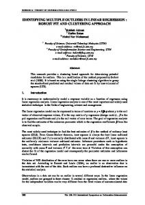
A simulation study is carried out to investigate the performance of the DFBETAc statistic for detecting outliers in the multiple circular regression model (2) based on equation (8). Four different sample size are considered, n = 30, 50, 70 and 100 with different value of 1 , 2 0.03, 0.03, 0.05, 0.05, 0.1, 0.1 and 0.3, 0.3 . The
vd* vd mod (2 ),
0
1
1
1
1
0
1
1
1
1
the DFBETAc j.i is calculated. If the values of DFBETAc d
,
is maximum and greater than the corresponding cut-off point, then the procedure has correctly detected the outlier in the data. The process is carried out 2000 times. The power of performance of the procedure is then examined by computing the percentage of the correct detection of the contamination observation at point d.
Step 4. Fit the generated circular data using the MCRM to give the parameter estimates of ˆλ Aˆ , Aˆ , Bˆ , Cˆ , Dˆ , Eˆ , Eˆ , Fˆ , Gˆ and Hˆ . 1 0 1 1 1 1 0 1 1 1 Step 5. Exclude the ith row from the generated circular data, where i = 1,…,n. For each i, repeat steps (4) for the reduced data set to obtain λˆ .
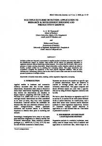
The simulation results are plotted in Figures 1-2. Figure 1 illustrates the power of performance of the DFBETAc detection method for n = 100 and four different values of 1 , 2 0.03,0.03,0.05,0.05,0.1,0.1 and 0.3,0.3 . It can be seen that the performance of the procedure is a decreasing function of 1 and 2 . This is expected as V1 j
j i
Step 6. Compute DFBETAc j.i for each i from equation (8). Step 7. Specify the maximum value of DFBETAc j.i .
and V2 j in equation (5) will fluctuate closer to the horizontal axis when 1 and 2 are closer to zero, and hence, better chance to detect the outlier even when is small.
The process is repeated 2000 times for each combination of sample size n and standard deviation 1 , 2 . Then the 5% upper percentiles of the maximum values of DFBETAc j.i are
9085
International Journal of Applied Engineering Research ISSN 0973-4562 Volume 13, Number 11 (2018) pp. 9083-9090 © Research India Publications. http://www.ripublication.com Table 1. The 5% upper percentiles of DFBETAc j.i statistic for 1 , 2 (0.3,0.3) at a = 2 sample size, n
A0
A1
B1
C1
D1
E0
E1
F1
G1
H1
20 30 40 50 60 70 80 90 100 120 150
3.72 3.82 4.22 4.26 4.84 4.93 5.34 5.43 5.51 5.57 5.69
2.55 2.67 2.96 3.00 3.36 3.37 3.77 3.80 3.93 3.97 4.20
2.55 2.92 3.06 3.01 3.08 3.08 3.08 3.18 3.26 3.39 4.06
2.43 2.44 2.44 2.63 2.54 2.75 2.71 2.90 3.05 3.08 3.22
1.91 1.94 2.18 2.29 2.33 2.36 2.62 2.69 2.71 2.83 2.88
4.45 4.53 4.56 4.88 5.05 5.13 5.18 5.55 5.70 5.71 5.89
2.77 2.83 2.92 3.13 3.21 3.37 3.47 3.60 3.62 3.71 4.12
3.65 3.54 3.58 3.59 3.62 3.64 3.75 3.82 3.87 3.99 4.07
2.92 2.98 2.93 3.17 3.00 3.40 3.47 3.69 3.96 4.10 4.20
2.09 2.24 2.16 2.23 2.41 2.42 2.41 2.96 2.57 2.68 2.89
Power
100
80
60
40
20
0
0.0
0.2
0.4
0.6
0.8
1.0
Figure 1. Power performance of DFBETAc statistic at n=100 Power
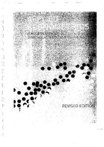
100 n=30 n.50 n.70 n.100
80
60
40
20
0
0.0
0.2
0.4
0.6
0.8
1.0
Figure 2. Power performance of DFBETAc statistic for 1 , 2 (0.1,0.1)
9086
International Journal of Applied Engineering Research ISSN 0973-4562 Volume 13, Number 11 (2018) pp. 9083-9090 © Research India Publications. http://www.ripublication.com
u1
PRACTICAL EXAMPLE
0
The multivariate eye data containing of 23 observations of glaucoma patients recorded using Optical Coherence Tomography at the University Malaya Medical Centre for three angles, namely the angle of the eye (v), the posterior corneal curvatures angles (u1) and the posterior corneal curvature when length of the perpendicular is fixed to 2 mm angels (u2) (See [10,13]). The least squares parameters estimates are , Bˆ1 11.685 , Aˆ1 7.089 Aˆ0 1.071, Cˆ1 2.969 , Dˆ1 1.452 , Eˆ0 3.124 , Eˆ1 9.963 , Fˆ1 16.536 ,
10 8 6 4 2
270
10 8
6
4
2
2
4
6
8 10
90
2 4 6
Gˆ1 4.227 , Hˆ 1 2.235 , ˆ1 0.1 , ˆ 2 0.1 and ˆ 0.987 . and thus the fitted model gives gˆ1 (u1 , u2 ) and gˆ 2 (u1 , u2 ) are as
8 10
180
follow
u2
(a) The posterior corneal curvatures angles
gˆ1 (u1 , u2 ) 1.076 7.089 cos u1 cos u2 11.685 cos u1 sin u2
0
2.969sin u1 cos u2 1.452 sin u1 sin u2
20 15
gˆ1 (u1 , u2 ) 3.124 9.963cos u1 cos u2 16.536 cos u1 sin u2
10
4.227 sin u1 cos u2 2.235 sin u1 sin u2 Further, the prediction of
vˆ j
5
270
given as
20 15 10
5
3.1246 9.9634 cos u1 cos u 2 16.5369 cos u1 sin u 2 vˆ arctan
equation (3) is given by ˆ u
1 n 2 ˆ u j 0.987 n j 1
toward
90
10 15 20
2.9691sin u1 cos u 2 1.4526 sin u1 sin u 2
10 15 20
5
4.2270 sin u1 cos u 2 2.2351 sin u1 sin u 2 1.076 7.0890 cos u1 cos u 2 11.6852 cos u1 sin u 2
and the concentration parameter
5
180
(b) The posterior corneal curvature when length of the perpendicular is fixed to 2 mm
u using
v 0
12.5 10
which suggest the data seem to be highly concentrated.
7.5 5 2.5
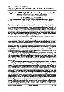
The goodness of fit test is performed by using Akaike information criteria (AICC) given by [14] .The AICC for MCRM is -51.06. This is supported by diagnostic plot. Figure 3 shows the simple circular histograms for multivariate eye data measured by three different angles. The posterior corneal curvatures angles concentrated around 90 , the posterior corneal curvature when length of the perpendicular is fixed to 2 mm angels around 37 , while the angle of the eye is more concentrated around 45 . While, Figure 4 (a) and (b) show the Q-Q plots for the residuals from two observational-models of the MCRM. The plot for 1 shows that most of the points are closer to the straight line except two points at the top right. Meanwhile, plot of 2 shows the points also relatively close to the straight line except one point at the right top of the plot. These points are corresponding to the outliers that might be existing in the data. They will be dealt with using numerical statistic, DFBETAc statistic in the next Section.
270
12.5 10 7.5 5 2.5
2.5 5 7.5 10 12.5
90
2.5 5 7.5 10 12.5
180
(c) The angle of the eye Figure 3. Simple Circular Histogram of eye data
9087
International Journal of Applied Engineering Research ISSN 0973-4562 Volume 13, Number 11 (2018) pp. 9083-9090 © Research India Publications. http://www.ripublication.com
(b) 2
(a) 1
Figure 4. Q-Q plot for residuals for contaminated data
estimates of Aˆ1 , Cˆ1 , Eˆ 0 , Fˆ1 , Hˆ 1 , ˆ1 and ˆ 2 in clean data are smaller than the contaminated data. Furthermore, most of the value of standard error for parameter estimates are smaller
(i) DFBETAc Statistic The DFBETAc statistic is applied to detect the possible outliers in the multivariate eye data. Since the number of multivariate eye data is 23, the cut-off point for this data is generated again and using the simulation program. The value of the parameter estimates for the 5% upper percentiles cut-off point for eye data is presented in Table 2.
than contaminated except for Cˆ 1 and Dˆ 1 . On the other hand, the concentration parameter, ˆ also increases from 0.987 to 0.992.
Table 3 presents the values of estimated parameters and the last two columns in the table give the number parameter estimates which exceed the corresponding cut-off points. The observations number 1, observation number 15 and observation number 23 are indicated as outliers, because they are exceeded the percentage of 0.4.
Figure 5 gives the Q-Q plots of the resulting residuals corresponding to the observational-models of the MCRM after removing those outliers from the multivariate eye data set. The plot shows all the points are close to the straight line comparing to the Figure 4, the Q-Q plots of resulting residuals corresponding to the observational before deleted the observations numbers 1, 15 and 23. That is denoting that the proposed method is the best fit for the data. Therefore, the standard errors for all parameters estimation become smaller after removing the outliers. This indicates a more accurate estimation and represent the method is perform well.
(ii) The Effect of Outliers on the Parameter Estimates In order to assess the detection of outliers, three observations; with numbers 1, 15 and 23 are identified and deleted. Then, the MCRM was refitted to get the parameter estimates. Table 4 summarizes the effect of excluding the outliers on the parameter estimates. The removal of observations with numbers 1, 15 and 23 significantly changes some of the estimated parameters of MCRM, where the parameter
Table 2. The cut-off point value for multivriate eye data Parameter Estimate
A0
A1
B1
C1
D1
E0
E1
F1
G1
H1
Cut-off point value
3.82
2.63
2.69
2.35
2.05
4.10
2.78
3.22
2.81
2.13
9088
International Journal of Applied Engineering Research ISSN 0973-4562 Volume 13, Number 11 (2018) pp. 9083-9090 © Research India Publications. http://www.ripublication.com Table 3. The values of the DFBETAc j.i statistic for multivariate eye data, n = 23 and the number influenced parameters Observation 1 2 3 4 5 6 7 8 9 10 11 12 13 14 15 16 17 18 19 20 21 22 23
A0
A1
B1
4.69 3.93 0.21 0.22 0.40 0.85 0.21 0.15 2.40 0.12 0.44 2.38 1.17 1.51 7.19 1.69 1.61 0.41 0.09 0.29 1.40 0.47 7.91
2.89 1.33 0.06 0.07 0.14 0.36 0.01 0.01 0.83 0.16 0.22 0.74 0.22 0.65 2.61 0.45 0.45 0.15 0.12 0.03 0.54 0.19 3.23
2.39 0.85 0.04 0.04 0.09 0.25 0.03 0.01 0.53 0.09 0.15 0.47 0.10 0.44 1.61 0.26 0.30 0.17 0.10 0.01 0.36 0.12 2.15
Parameter Estimate C1 D1 E0 E1 8.69 2.93 0.16 0.08 0.41 1.38 0.41 0.24 1.63 0.12 0.71 2.22 0.37 1.72 0.75 0.34 1.20 2.61 0.56 0.25 1.52 0.06 6.48
7.47 0.38 0.02 0.10 0.07 0.65 0.54 0.07 0.25 0.02 0.35 0.30 1.20 0.46 4.09 0.97 0.18 2.56 0.46 0.04 0.39 0.28 2.91
5.74 5.53 0.27 4.60 2.09 1.12 0.22 0.11 2.48 0.04 0.53 3.48 1.14 1.63 4.51 1.96 0.95 0.52 0.10 0.30 1.47 0.87 4.65
2.99 1.88 0.08 1.39 0.70 0.48 0.01 0.01 0.86 0.06 0.27 1.08 0.22 0.68 1.64 0.52 0.27 0.19 0.13 0.03 0.57 0.34 3.05
F1
G1
H1
0.29 1.20 0.05 0.85 0.46 0.33 0.03 0.01 0.55 0.03 0.19 0.68 0.10 0.45 1.01 0.30 0.18 0.21 0.10 0.01 0.38 0.22 0.97
10.64 4.12 0.21 1.72 2.10 1.83 0.43 0.17 1.68 0.05 0.86 0.47 0.36 1.78 3.25 0.39 0.71 3.32 0.57 0.26 1.60 0.11 2.91
9.14 0.53 0.02 2.06 0.35 0.86 0.55 0.05 0.26 0.01 0.42 0.43 1.17 0.48 2.57 1.12 0.11 3.25 0.47 0.04 0.41 0.52 2.75
Influenced parameters Number Percentage 8 3 0 1 0 0 0 0 0 0 0 0 0 0 5 0 0 4 0 0 0 0 8
0.8 0.3 0 0.1 0 0 0 0 0 0 0 0 0 0 0.5 0 0 0.4 0 0 0 0 0.8
Table 4. DFBETAc statistic of multivariate eye data without observations number 1, 15 and 23 , n=20 Parameter estimates
Contaminated data -1.0716
Standard error 1.0818
Clean data (case1,15 and 23 deleted) 0.8369
Standard error 0.3518
7.089
3.2265
1.5022
1.4217
-11.685
4.9832
-2.6209
2.4508
2.9691
1.2998
-0.9197
1.3060
-1.4526
1.7862
1.1060
1.8805
3.1246
0.9154
0.6566
0.2144
-9.9634
2.7301
-1.8945
0.8665
Fˆ1 Gˆ
16.5369
4.2167
3.29208
1.4937
-4.227
1.0998
0.1303
0.7960
Hˆ 1
2.2351
1.5114
-0.1061
1.1461
ˆ 1 ˆ 2 ˆ
0.136 0.115 0.987
0.285 0.230 -
0.103 0.107 0.992
0.079 0.094 -
Aˆ 0
Aˆ1 Bˆ
1
Cˆ 1 Dˆ
1
Eˆ 0 Eˆ
1
1
9089
International Journal of Applied Engineering Research ISSN 0973-4562 Volume 13, Number 11 (2018) pp. 9083-9090 © Research India Publications. http://www.ripublication.com
(b) 2
(a) 1
Figure 5. Q-Q plot for residuals without observations numbers 1, 15 and 23 for contaminated data
CONCLUSION This paper proposed the DFBETAc statistic by extending the DFBETAS statistic in linear to the multiple circular regression model, where the model shows appropriate features as the linear case. The cut-off points and power of performance are obtained via simulation. The proposed method was applied on eye data, and three possible outliers have been identified which are similar to observations detected by dataset of outliers as found in [10].
[8]
S. Ibrahim, A. Rambli, A.G. Hussin, and I. Mohamed. "Outlier detection in a circular regression model using COVRATIO statistic." Communications in StatisticsSimulation and Computation 42, no. 10, 2013.
[9]
A. Rambli, R. M. Yunus, I. Mohamed, and A. G. Hussin. "Outlier Detection in a Circular Regression Model." Sains Malaysiana, 44, no. 7, 2015.
[10] N.A. Alkasadi, S. Ibrahim, M.F. Ramli, and M.I Yusoff. "A Comparative Study of Outlier Detection Procedures in Multiple Circular Regression." In AIP Conference Proceedings, vol. 1775(1), “AIP Publishing”, 2016.
REFERENCES
[11] D.A. Belsley, E. Kuh, and R.E. Welsch, “Regression Diagnostics: Identifying Influential Data and Sources of Collinearity”. New York: John Wiley & Sons, 1980.
[1]
D.R. Bacon. "A Maximum Likelihood Approach to Correlational Outlier Identification." Multivariate Behavioral Research 30.2 (1995): 125-148.
[2]
D.C. Montgomery, A.P. Elizabeth, and G.G. Vining. “Introduction to Linear Regression Analysis”. Vol. 821. John Wiley & Sons, 2012.
[3]
O. Torres-Reyna. “Linear regression using Stata. In Statistic Handout”, Princeton University, 2007
[13] S. Ibrahim. “Some Outlier Problems in a Circular Regression Model”, PhD Thesis, University of Malaya, 2013.
[4]
A.H. Abuzaid, A.G. Hussin, and I. Mohamed. "Identifying Single Outlier in Linear Circular Regression Model Based on Circular Distance." Journal of Applied Probability and Statistics3, no. 1, 2008.
[14] U. Lund, “Least circular distance regression for directional data”, Journal of Applied Statistics, 26 (6), 723-733, 1999.
[5]
A. Rambli, A., I. Mohamed, A.H. Abuzaid, and A.G. Hussin. "Identification of influential observations in circular regression model." In Proceedings of the Regional Conference on Statistical Sciences, 2010.
[6]
A.H. Abuzaid, I. Mohamed, A.G. Hussin, and A. Rambli. "COVRATIO statistic for simple circular regression model." Chiang Mai J. Sci 38, no. 3, 2011.
[7]
A.G. Hussin, A.H. Abuzaid, A.I.N. Ibrahim, and A. Rambli. "Detection of outliers in the complex linear regression model." Sains Malaysiana 42, no. 6, 2013.
[12] S.R. Jammalamadaka, and Y.R. Sarma. “Circular Regression. In: Matsusita, K”, ed. Statistical Science and Data Analysis. Utrecht: VSP, 1993.
9090