we will focus on a multispectral image gradient estimation. The image gradient is ... function. The image gradient forms the base for many other edge detection algorithms like the Can- ..... very large (e.g. gigapixel or hyper-spectral datasets).
Remote Sensing and Geoinformation not only for Scientific Cooperation
Lena Halounová, Editor EARSeL, 2011
A Modular Framework for the Comparison of GradientBased Multispectral Edge Detectors Benjamin Seppke, Leonie Dreschler-Fischer and Dennis Hamester University of Hamburg, Department of Informatics, Cognitive Systems Laboratory, Hamburg, Germany; {seppke, dreschler, 7hameste}@informatik.uni-hamburg.de Abstract. The aim of this research is to determine an accuracy assessment of different multispectral gradient-based edge detectors. We will present and evaluate three different approaches: the mean-, the maximum- and the multispectral gradient approach. The mean approach determines the overall gradient as the arithmetic mean of all (band-wise) gradient vectors, whereas the maximum approach selects the gradient vector of maximum length. The first two algorithms that are heuristically motivated, the multispectral gradient approach can be derived mathematically from the single band gradient-based approach and thus is very interesting to investigate (see [1]). To compare and evaluate the algorithms, we designed a modular framework that is based on generic programming and the VIGRA computer vision library [2]. We discuss the framework's architecture in more detail to demonstrate the flexibility. For the evaluation we synthesized artificial images where we know the exact location and occurrence of edge elements (evaluation by means of dedicated techniques [3]). The evaluation shows that in many cases the naive mean approach does not lead to satisfactory results. In some cases, the maximum- and the multispectral gradient approach are almost on the same level of detection quality. In other cases the multispectral gradient approach outperforms the other two approaches. Complementary to the quantitative evaluation, we present the application of the algorithms to Landsat 7 ETM+ satellite multispectral imagery of coastal and urban areas taken from the public Landsat Archive. Keywords. multispectral imagery, gradient operators, edge detection, computer vision.
1. Introduction The accurate detection of edges or boundaries in digital images has been under investigation since the very beginning of computer vision and image processing. A variety of tasks require a good detection of edges, e.g. 3D-scene reconstruction, image segmentation or motion detection. Better lowlevel edge detection thus yields better results in the succeeding higher-level algorithms. In this work we will focus on a multispectral image gradient estimation. The image gradient is defined as the vector of the partial first derivatives and describes the rate of local intensity change of an image function. The image gradient forms the base for many other edge detection algorithms like the Canny edge detector [4] or segmentation algorithms like the watershed transform [5]. We will start with the definition of such a gradient for the case of grey-value (single channel) images, where many algorithms have been developed over the last decades. The situation becomes more involved in case of multispectral imagery. The main question is how to integrate the information of each spectral channel into one gradient estimation algorithm, which determines a closed representation for multispectral images. Recent studies have lead to many approaches, which seem to be plausible, but are – more or less – heuristically motivated (see e.g. [6]). In addition, many multispectral gradient-based approaches have just been evaluated qualitatively. Only few authors have performed a quantitative evaluation yet (see e.g. [3], [6]).
Seppke, Dreschler-Fischer, Hamester: A Modular Framework for the Comparison of Gradient-Based Multispectral Edge Detectors
We will describe and evaluate three different approaches for the gradient estimation using multispectral images in this work. Each approach uses a different strategy to estimate and integrate the single-channel edge information. Beside the implementation of two heuristically motivated algorithms, the mean- and maximum gradient approach, we are focusing on a mathematically motivated approach, which has been proposed by Di Zenzo [7] and further investigated by Drewniok in [1] and [8]. This approach extends the classical discrete gradient operator formally to multispectral images and thus lets us expect promising results. One main advantage is the generality of the algorithm’s definition, which allows for an extension of commonly known gradient operators to multispectral images. This unique property leads to a very modular algorithmic design. We have implemented three different interchangeable approaches by means of a modular framework. All algorithms are sharing a common interface and hence can be modularly replaced and evaluated. Beside the presentation of the results of each algorithm, we emphasize on a general evaluation by means of e.g. the accuracy of edge localization than on subjective measures. To do this quantitative evaluation, we use a synthetic image and analyze the errors made when the image noise increases. To measure the quality of the edge detectors, we use the technique introduced by Venkatesh in [3] but extended the criteria to take an orientation error of the computed edgels into account (see [9]). We will also show the results of all approaches applied to Landsat 7 ETM+ data, for urban and coastal areas. In the next chapter, we will formally introduce the definitions of images, multispectral images and edges as well as differential edge detection algorithms. These algorithms will then be used in the subsequent chapter to compute the results. 2. Methods Before we are going into details about the methods’ definitions, we first want to introduce with the definition of an image. We start by defining a continuous image I of n channels
I : R ! R " Rn
(1)
The image I is defined as function, which assigns an n-dimensional intensity-vector to each spatial position. We assume that the image function is differentiable over the whole domain. For the special case of a single channel image an image is defined as a function, which maps to a real value, not to a vector. Although, we have in practice no continuous images, these definition is a very well tractable mathematically background for the gradient definition, which forms the base for the edge detectors we present in the following section. Subsequently, we need to define the digital image, too: n I digital : N ! N " Rdiscrete # Rn
(2)
As we can observe from the upper definition, the image’s domain and image’s image set are both discretized during the digitalization. This discretization consists of two steps: the sampling, which discretizes the image’s domain, and the quantization, which discretizes the image’s image set. Consequently the differential approaches we are focusing on, can all be defined continuously but need to be discretized when applied to digital image data.
2
Seppke, Dreschler-Fischer, Hamester: A Modular Framework for the Comparison of Gradient-Based Multispectral Edge Detectors
2.1. Single channel gradient definition Based on the continuous image definition of eq. (2), we can define the edges in single channel images as strong intensity changes in a spatially local environment around a given pixel. If the degree of intensity change is above some given value, we may call this pixel an edge element (edgel). The definition of eq. (2) allows for a more mathematically motivated spatially change description by means of the partial spatial derivatives:
!I =
(
Ix
Iy
)
T
where I x =
!I !I , Iy = !x !y
(3)
This results in a gradient vector for each image pixel. Local extremes of this vector correspond to image positions where the images gray values vary the most. To describe the strength of the images gradient, many measures can be defined. Roberts e.g. proposes to use the two-dimensional Euclidean vector length as a scalar measure of intensity change. The length in conjunction with the orientation of the vector yields to another commonly used representation: L = !I
and ! I = atan2 ( I x , I y )
" !1 x $ tan ( y ) where atan2(x, y) = # $ tan !1 ( xy ) + !2 %
& y>0 $ ' else $ (
if
(4)
Based on the continuous definitions, many discretizations for partial first order derivatives of an image have been developed. A comparison can e.g. be found in [6]. In this work, we will focus on the discretization of the first spatial derivative by means of a separable convolution with derived Gaussians of first order. This approach has some advantages over other approximations and results in a very fast gradient estimation (see [10]). After the formal description and introduction of a spatial derivative estimation for one grey-value image, we will describe three different combination approaches of single band information in the following section.
Figure 1: The image’s gradient for a single channel image. Upper panel: the gray scale image and the resulting partial derivatives Ix and Iy , which form the gradient information. Lower panel: the gradient magnitude and angle representation. The derivatives have been computed using a Gaussian first order kernel with ! = 1
3
Seppke, Dreschler-Fischer, Hamester: A Modular Framework for the Comparison of Gradient-Based Multispectral Edge Detectors
2.2. Gradient definitions for multispectral images Another view on multi-channel images, which deviates from eq. (1), is to define a multi-channel image as a stack of n single channel images. Following this view, we are able to compute the single channel gradient for each channel separately. Let !I c denote the single channel gradient for the cth channel of the image. We can now generalize the single channel gradient operator of eq. (3) for the case of multispectral images:
" !I % " (I1 1 $ ' $ (x !I = $ ! ' = $ ! $$ !I '' $ (In n # & $# (x
% ' ! '= J ' (I n1 ' (y & (I1 (y
(5)
The matrix J contains the derivatives of each gradient component and is the commonly known Jacobian matrix. We will recall this matrix in more detail in the multispectral gradient approach at the end of this section. Based on the above definition, the main challenge is the integration of the components of the resulting vector. This can be seen analogously to the combination of an x- and yderivative to one scalar (the length) for the single channel case in eq. (4). We will now start with an introduction of the approaches we selected for this work: the mean-, maximum-, and multispectral gradient approach. The first approach combines the different gradient information of each channel using the arithmetic mean: !I =
1 n " !I c n c=1
(6)
The mean operator suffers from mutual extinction of opposing gradient. Although this approach is very basic and may yield to good results when the variation of the vectors’ directions do not differ too much, we will now present a second approach, the maximum approach, which does not suffer from anti correlated vectors:
max(!I ) = argmax !I c
(7)
c
Although this operator solves the mutual extinction problem of the mean operator, all information of the non-maximum vectors is lost. Two cases, the advantages and disadvantages of the mean- and maximum approaches, are shown in fig. 2.
Figure 2: Problems of the mean and maximum approach. Left: the mean approach fails, because all blue vectors sum to the negative of the red vector, and thus the mean is zero. Right: the maximum approach selects the singleton red vector although there is more evidence for the opposite directions (in blue).
4
Seppke, Dreschler-Fischer, Hamester: A Modular Framework for the Comparison of Gradient-Based Multispectral Edge Detectors
After the presentation of the mean- and maximum approach, we will define a third approach, which is less heuristically but more theoretically founded. The aim of this operator is to assign one scalar value to each the strength and angle of the multispectral image. We refer to this approach as the multispectral gradient approach, because it uses all partial derivatives in conjunction to estimate the largest difference vector. We will present the approach very briefly, but want to mention that more information can be found in [1], [7] and [8]. Let us assume, that there exists a direction vector d which corresponds to an angle ! in the following way:
! ! cos(! ) $ & d =# # sin(! ) & " %
(8)
The multispectral derivation in this direction can then be expressed by: ! ! ! d I = !I " d = J " d
(9)
The matrix J is the Jacobi matrix from eq. (5). To define magnitude of change, Drewniok proposed the use of the squared Euclidean distance of the resulting vector (see [1]). This approach turns to be mathematically attractive as the amount of squared change is given by: !2 !T ! ! ! (10) L2 (! ) = J ! d = J ! d ! J ! d = d T ! ( J T ! J ) ! d
(
) (
)
Independently of the channel count, this results in a symmetric 2!2 matrix of the following coefficients in between the direction vector:
" a a J ! J = ( ) $$ a11 a12 # 21 22 ! ! Since d T ! ( J T ! J ) ! d T
% ' ' &
2
2 n # n " " !I % !I !I & !I % where a11 = ($ i ' , a12 = a21 = )% i " i ( and a22 = ($ i ' (11) i=1 # !x & i=1 $ !x !y ' i=1 # !y & n
is the Rayleigh-quotient of the matrix ( J T ! J ) , the extremes of this quo-
tient are given by the eigenvalues of the matrix. The magnitude and direction of strongest change can be estimated by the largest eigenvalue and eigenvector of this matrix. Additionally, the solution of such an eigenvalue-problem is trivial because there exists an analytical solution:
(
!1,2 = 12 ( a11 + a22 ) ±
( a11 ! a22 )
2
)
+ 4a122 , where !max = !1 and !min = !2
(12)
Using this equation, we can determine the amount of change by means of the largest eigenvalue. The direction of change can now be defined using the corresponding eigenvector equations:
! = atan2 ( !max ! a11 , a12 ) using atan2 of eq. (4)
(14)
Due to the definition of the multispectral change by means of squared lengths in eq. (10), the angle ! cannot be determined in the complete interval of [-180°, 180°) but in a half circle of: [-90°, 90°). This is caused by the quadratic term of eq. (10), which makes it impossible to decide whether a vector points to the first or third quarter (and to the second or fourth quarter respectively). To solve this, different approaches are possible. To save computing time, we propose the use of a back-face voting algorithms. We compute the dot product between the computed direction and each channel’s gradient direction and sum its signs (-1 or 1) up to one single value. If the result is positive, the vector already points into the correct direction. If the result is negative, we flip the computed vector’s direction to get the final direction. 5
Seppke, Dreschler-Fischer, Hamester: A Modular Framework for the Comparison of Gradient-Based Multispectral Edge Detectors
Figure 3: Example for the multispectral gradient algorithm: the gradient vectors for different channels (green), derived axis (red), and finally derived direction vector via the voting algorithm (blue).
2.3. Evaluation method After the definition of three different gradient computation methods, we will present the used evaluation method to compare the results of the different operators. We use an extended version of the approach proposed by Venkatesh und Kitchen [3]. The evaluation starts with an ideal edge definition image and pose the question, which kinds of errors may have been made by edge detection operators. Venkatesh und Kitchen conclude with a set of four different error classes: • • • •
False positive (FP) An edgel has been detected although there is no edgel in the reference. False negative (FN) The detector missed the detection of a given edgel. Multiple detection (MD) An edge was detected more than once. Localization (LOC) The edgel has been detected, but slightly displaced to the reference position.
For each of these error classes, a single error measure is introduced according to the abbreviations in the above list. The original definition of these errors can only be applied to a very small subset of edgels namely horizontal or vertical edges. To use this approach in conjunction with arbitrary edge directions, we extended it and added the estimation of a direction error (DIR) (see [9]). Using the extended version of the above algorithm, we are able to compare the errors made on various gradient images edges, independent of the direction and connectedness. 3. Results The results presented in this section have been computed using a prototypical framework, which is mainly written in Python using the SciPy / NumPy [11], Matplotlib [12] and VIGRA [2] packages. For the single channel gradient estimation algorithm, we use the graussianGradient function of the VIGRA (see [2]). Although this framework is just prototypical, it already encapsulates the different gradient operators, so that they can be freely interchanged due to their common interfaces. Figure 4 shows a chart of the current framework. The general structure will remain unchanged no matter, which programming language has been chosen. 6
Seppke, Dreschler-Fischer, Hamester: A Modular Framework for the Comparison of Gradient-Based Multispectral Edge Detectors
For the results, we have selected two settings: a quantitative evaluation of all approaches and an application of these approaches to real world multispectral image data.
Figure 4: The proposed framework. Due to the same data produced by all multispectral gradient operators, it is highly flexible.
3.1. Evaluation of the proposed method To evaluate the three gradient estimation approaches, we have selected a very basic but appropriate test image: circle. The image is a three channel RGB-image of dimensions 129x129 pixels and contains a large yellow circle in front of a blue background. This setting is insofar advantageous as it contains edges of all directions, and not just horizontal or vertical ones. This is much closer to real world images, where the edges are usually not constraint to two directions. The boundary between the fore- and background has a contrast of 255 gray values. The image and the reference boundary is shown in fig. 5.
Figure 5: The used test image circle (left) and the reference boundary position image (right).
One of the most important properties of an edge detection algorithm is the robustness to noise. All presented approaches are based on first order derivatives, so we expect a good comparability between the approaches. Contrary to second order derivative filters like Laplacian based filters, the basic noise robustness should be better for the approaches presented herein. We will compare the edge detection results of the different approaches while decreasing the signal to noise ratio (SNR) of the image using additive noise. To compare the results with the reference edgels, we extracted the edgels from the resulting multispectral gradients by means of local maxima of the gradient magnitude.
7
Seppke, Dreschler-Fischer, Hamester: A Modular Framework for the Comparison of Gradient-Based Multispectral Edge Detectors
-/3+(45):+%&3,&55%6&:; -/3+(!
#!
@!
8!
0!
1!
?!
=!!
!'-,(+.(/0-)%',$1 !'-,(-&&0+-*8 !-;%!"!(-&&0+-*8 /0-)%',$(!-;%!"!
395 !"#$%&#'()'$'*$%+,
!"8
!"#$%1&'*$0-#(-&&0+-*8 !"#$%BC'*$+0(-&&0+-*8
6
*&#').9)!"#$%&'(: *&#')#--".#/0 *#+%*,*)#--".#/0 !"#$%&'()*#+%*,*
128 9#5:&)'&!#(%7&
!"1 2&34),564(+(7)
*,5(%:-&/("#5)#--".#/0 *,5(%67&/(.")#--".#/0
4
-)&*,62,$%&'()*+4 -)&*,&55%6&:; -&.(-/-,&55%6&:; $%&'()*+,-&.(-/-
1
41
C1
1
ABC
?1
31
;1
81
=1
411
3
63
:3
23
A3
@AB !6789:&")8'#7%#&&'(#)* !67890
"*+
,>/
"*,
,
" +,
2,
1,
/,
-, 345
@3
53
43
633
0,
;,
.,
?,
+,,
>"
!""
-&)'.)//$#)01 -)=%-:-.)//$#)01
"*6
,>2
,
?3
-:;(%