A Multi-Model Approach for Anomaly Detection and ...

Published in IEEE 06/2013; DOI:10.1109/ICPHM.2013.6621426 In proceeding of: Prognostics and Health Management (PHM), 2013 IEEE Conference on

A Multi-Model Approach for Anomaly Detection and Diagnosis Using Vibration Signals Victor B˘al˘anic˘a⇤ , Linxia Liao† , Heiko Claussen‡ and Justinian Rosca‡ Siemens Corporation, Corporate Technology Princeton, NJ USA ⇤ Email: [email protected] † Email: [email protected] ‡ Email: [email protected] § Email: [email protected]

Abstract—Continuous vibration monitoring of mechanical roller bearing parts potentially reduces machine downtime through timely prediction and diagnosis of abnormal events. Despite the progress made in the literature, challenges remain in how to assess performance related information for maintenance decision-making from large data streams. Furthermore, since roller bearings operate under various regimes (e.g., speed and load), it is not trivial to consider the effect of regime changes in the modeling in order to reduce false alarms. The paper describes a multi-model approach to monitor the condition of roller bearings under different operating regimes. Two modeling approaches for anomaly and degradation monitoring are proposed to automatically retrieve information from the data. A self-organizing map (SOM) and a support vector machines (SVM) are used comparatively for the evaluation of a bearing degradation in time (i.e., a dynamic health indicator) and for the determination of changes in the tracked features. The proposed method is validated using data from multiple bearings of the same type. Keywords:bearing diagnosis; anomaly detection; vibration analysis; support vector machine

I. I NTRODUCTION Real-time bearing condition monitoring is key for acquiring diagnosis information regarding bearing health at different operation regimes and deriving business effective decisionmaking for optimized maintenance, long-term availability and increased reliability. Simultaneously, bearing supervision can provide continuous data streams for improving the bearing control strategy for changing regimes avoiding operation inadvertences, fatal breakdowns and even preventing accidents. Roller bearings are among the most common failure points of the wide variety of mechanical systems used everywhere in industry such as gearboxes, compressors, turbines, pumps, motors and generators. Statistical data shows that 90% of faults which occur in rolling bearings are due to cracks in inner and outer race and the rest are cracks in balls or cage [1]. Though sensing the level of strain, acoustics, temperature, voltage, current and electrical power can provide information on bearing condition (cracks, chips, flaws, distortions, rust, corrosion, wear, looseness, improper riveting [2]) depending on the application/system, the most powerful tool for monitoring and predicting bearing health remains the vibration analysis [3]. A roller bearing produces unique vibration frequencies specific for its four components: inner race, outer race, ball spin and

cage. Their amplitude can be mathematically derived [4], [5], [6] making an indication of their health condition possible by comparing the actual measured vibration spectrum with the ideal one and recognizing bearing faults. Roller bearing defect diagnosis by employing artificial intelligence techniques has been widely studied in the literature, extensive reviews being offered by [3], [7], [8] and others. Comparing two outstanding and application effective techniques in diagnosing rotating machineries, i.e., the artificial neural networks (ANNs) and the support vector machines (SVMs), the latter proves to attain higher accuracy and a better generalization power for a smaller number of training samples when used in non-linear pattern recognition tasks [8], [9]. This paper describes a multi-model approach for monitoring and diagnosing the health of bearings under different operation regimes such as speed, torque, stress and/or load. Two modeling approaches for anomaly and degradation detection are proposed to automatically retrieve information by analyzing features derived from roller bearings vibration data. A selforganizing map based method is used for the definition and evaluation of a dynamic health indicator of a roller bearing and for the determination of significant changes in the tracked features. Furthermore, a support vector based method is used comparatively for validation of the SOM results, though SVMs are mainly used in classification and feature selection tasks. Specifically, the proposed multi-model approach implies the use of separate models for each operating regime in order to track the degradation of the roller bearing for each individual regime. Simultaneously, computing the contribution factors of selected features and comparing them to the training feature set can help field engineers diagnose the root causes of the degradation. The models are trained taking into account historical records and are validated using data from multiple bearings of the same type. The approach shows potential in timely and reliably predicting incipient bearing faults, saving time and costs of maintenance while increasing availability. II. P ROPOSED APPROACH Roller bearing fault diagnosis can be approached by using either a physics-based model or a data-driven model. The physics-based approach requires a very good insight into the

mechanics of the bearing and can produce accurate prognostic information when designed properly. However, it takes tremendous effort to acquire an accurate model for different regimes of operation that usually lacks in adaptability when diagnosing different types of bearings. On the other side, the data-driven statistical model can provide robust and reliable prognostic information when sufficient data and expertise is available, but the diagnostics output is less intelligible/comprehensible. The model presented here is designed for large-scale and diverse uses and implements the data-driven approach. A. Multi-Model Approach The proposed methodology divides the problem into multiple regimes and addresses each regime in a divide-andconquer approach, alleviating the high complexity of modeling boundaries for a combination of multiple operating regimes. Figure 1 shows the analysis workflow. A similar approach can be found in [11]. First, the historical data of the power level is collected to identify the operating regimes. Second, a feature extraction method is applied to vibration sensor signals to extract diagnosis-relevant features.

algorithms use data labeled as normal operation (no fault in the maintenance log) for each regime as training data in order to detect unexpected faults and monitor degradation of bearings in the test data via a health indicator. Multiple SOM and SVM models are trained separately for each specific operating regime. The last step of the workflow implies the application of the trained SOM and SVM based models on the test vibration data collected from for different roller bearings of the same type. The health indicator for the new data is calculated to track the degradation of bearings over time. If an anomaly of the bearing is observed at a certain time stamp, the contribution of each feature to the anomaly is calculated and compared to the training data. The changes seen in features can enrich the potential of finding and understanding the root causes of the bearing and helping field engineers with fast diagnosis. B. Degradation Monitoring Using SOM The method adopted for degradation monitoring is the selforganizing map (SOM) [13]. In unsupervised training the SOMs are capable of learning patterns of behavior existing in the input data. For degradation monitoring of bearings or other systems, an unsupervised SOM is trained based on normal/baseline data that reflects the normal behavior of the investigated system. The applications of SOM also include anomaly detection and diagnosis as described in [14]. A short introduction to SOM and the definition of minimum quantization error (MQE), used as the machine health indicator to indicate the degradation level, are given below. Let x = [x1 , x2 , ..., xp ] denote a p-dimensional input set and wb = [wb1 , wb2 , ..., wbp ] represent the weight vector of neuron b = 1, 2, ..., N , where N is the number of neurons of a SOM. The best matching unit (BMU) wm is defined by the neuron whose weight vector is the closest to the input vector x. The distance from x to wm is given by |x

Fig. 1.

Flowchart of data analysis

Third, a feature selection method is applied to the extracted features. The purpose of feature selection is to identify the critical features that can provide the most useful information, while reducing noise and eliminating redundancy. The feature reduction method does not reduce the number of sensors, but projects the original feature space into a new feature space where different faults can be identified more clearly. More information on feature reduction can be found in [12]. The feature space after feature selection/reduction is used as input for algorithms performing anomaly detection, diagnosis and degradation monitoring. A training procedure is applied to the SOM and SVM based models using data for each of the operating regimes. The

wm | =

min

b=1,2,...,N

{|x

wb |}

(1)

and represents the minimum quantization error (MQE). While training a SOM in an unsupervised manor, the weight vectors that are topographically close to an input vector are updated according to a defined neighborhood kernel function, resulting in a local relaxation or smoothing effect on the weight vectors of neurons in that neighborhood. Similar to a neural network, the following learning rule is applied wb (t + 1) = wb (t) + (t)hb (t)(x

wb (t))

(2)

where t is the discrete-time coordinate, (t)is the learning rate and hb (t) is the neighborhood kernel function. The training iterates until a predefined stop criterion is met. The degradation level of a new observation is computed by testing the new input vector with the trained SOM and finding the BMU to the input vector. The Euclidian distance of the input vector to its BMU is calculated as the health indicator.

C. Anomaly Detection Using SVM SVMs are classically used in classification tasks. The approach in this paper is to use a SVM in monitoring degradation via a health indicator for validation purposes of the SOM results. The linear and non-linear classification power in high dimensional spaces of the support vector machines (SVMs) is derived from their ability to create an optimal separation hyper-plane between the classified data sets in such way that the distance between the boundaries of the classes is maximized. The data points in each class used to define the so-called margin are known as support vectors. A 1-class SVM is a machine that is trained on data belonging only to a single ’normal’ class and is used to perform classification tasks of input data into either the ’normal’ or the ’abnormal’ diagnosis class. Assuming S a training data set given by S = {xi , yi }M i=1

(3)

where xi ✏IRp with i = 1, ..., M is one of the M training data points of dimensionality p and yi ✏{ 1, +1} its corresponding binary class label, the SVM classifier that finds an optimal hyper-plane satisfies the following two inequalities: wT '(xi ) + b

1,

if

yi = +1

(4)

wT '(xi ) + b < 1,

if

yi =

(5)

1

where w✏IRN is a weight vector and the bias b is a scalar. If all training data points verify the previous inequalities, the classes are linearly separable [15]. The non-linear function '(·) denotes a fixed feature-space transformation which can map the input space to a high dimensional feature space. Therefore, determining the optimal hyper-plane in the linearly separable case translates in solving the following constrained optimization problem: 1 arg min wT w 2 w subject to: yi (wT '(xi ) + b)

(6) 1, i = 1, ..., N

If some data points in S do not verify the inequalities in Eq. (4) and (5) the SVM becomes linearly not separable and the determination of the optimal decision hyper-plan translates in solving the following constrained optimization problem: 1 arg min wT w + C⌃N i=1 ⇠i w,b,⇠ 2 subject to: yi (wT '(xi ) + b) ⇠i

(7) 1

⇠i

0, i = 1, ..., N

where the ⇠i variables are slack variables which are needed to allow misclassifications in the set of inequalities. In order to solve the above constrained optimization problem, a set of Lagrange multipliers ↵i is introduced. The Lagrange multipliers ↵i are then determined by means of the following optimization problem (dual problem):

1 N N ⌃ ⌃ ↵i ↵j yi yj xTi xj , (8) 2 i=1 j=1

arg min Q(↵) = ⌃N i=1 ↵i ↵

subject to: ⌃N i=1 ↵i yi = 0, 0  ↵i  C, i = 1, ..., N.

If 0  ↵i  C, the corresponding data points are called support vectors (SVs). When a linear boundary in the input space is not enough to separate the classes properly, it is possible to create a new hyper-plane that allows linear separation in the higher dimension. In a SVM, this is being achieved by a transformation '(x)✏IRM , where M > N , that performs the nonlinear mapping into a higher dimensional Hilbert space. If K(x, xi ) is the inner product kernel defined by K(x, xi ) = K(xi , x) = '(x)T '(xi )

(9)

the above dual optimization problem is given by 1 N N ⌃ ⌃ ↵i ↵j yi yj K(x, xi ) 2 i=1 j=1 (10)

arg min Q(↵) = ⌃N i=1 ↵i ↵

subject to: ⌃N i=1 ↵i yi = 0, 0  ↵i  C, i = 1, ..., N.

The kernel K(x, xi ) is required to satisfy Mercers theorem [17]. Therefore the unseen data is classified as: y = {1,

f or

m(x)

0

or -1,

f or

m(x) < 0} (11)

where the decision function can be expressed as m(xi ) = yi (⌃N j=1 yj ↵j K(xi , xj ) + b)

(12)

The most common used kernel function, K(x, xi ), are the following choices, [16]: • Radial-basis function: K(x, xi ) = exp( gkx xi k2 ), g > 0 • Polynomial: K(x, xi ) = ( xT xi + r)d , > 0 • Sigmoid: K(x, xi ) = tanh( xT xi + r). D. Degradation Monitoring Using SVM In unsupervised training SVMs are capable of learning patterns existent in the input data. For degradation monitoring of bearings or other systems, an unsupervised SVM is trained based on normal/baseline data that reflects the normal behavior of the investigated system. A new observation is tested with the trained SVM and the distance to the baseline is calculated as a machine health indicator, namely the degradation level. A short introduction on how to use SVMs to provide the machine health indicator (or degradation level) and the corresponding contribution factors of features is given below. Let every data point xi = xkij = [xki1 , xki2 , ..., xkip ] describe a vector containing p features, where j = 1, 2, ..., p and k = 1, 2, ..., l describes the available operating regimes.

For any specific operating regime k, the trained SVM dek k k k livers a set of support vectors wc = wcj = [wc1 , wc2 , ..., wcs ], with c = 1, 2, ..., s, that describe the separation hyper-plane between the normal and abnormal roller bearing behavior. The proposed method determines the health indicator Hik of the roller bearing (or of any other investigated machine) for a certain operating regime k. This is done by computing the minimal distance of a test data point xi , that is normalized using the training dataset, to the SVM separation hyper-plane, that was previously determined in the training procedure. If the distance from a data point xi to the nearest support vector wd is given by the Euclidian distance as in

then

Hik

is given as

distki = |xki

Hik =

wdk |,

min {|xki

c=1,2,...,s

wck |}.

(13) (14)

Simultaneously, a contribution vector for all features can be defined for every health indicator Hik of the test data point xki . The contribution vector is computed by subtracting the values of the features between the test data point xki and the closest support vector wdk in order to account for and give insight into the root cause of the degradation level. This is given by k Cij = xkij

k wdj ,

with j = 1, 2, . . . , p.

(15)

The determined feature contribution vector Cik can further help experts to determine and quickly diagnose known defects or easily correlate feature changes to physical roller bearing observations and degradation levels. III. M ODEL VALIDATION Vibration data of roller bearings is acquired using two types of accelerometers as structural vibration sensor: one capturing data in the range of 20g and the frequency band 0Hz-1kHz and the other in the range of 6.4g and the frequency band 0.1Hz-8kHz. Both sensor types are attached to each bearing in order to provide accurate vibration measurements. A. Signal Processing, Feature Extraction and Selection The data acquisition controller for the roller bearings provides raw time data of approximately 1-2 seconds length. The available data ranges from June 2011 to October 2012. The following feature extraction methods have been performed on the time domain data: root mean square, mean value, crest factor, skewness and kurtosis. The following features have been computed on the frequency spectrum: energy bands of width 100 Hz and the energy bands for the rotation speed and for multiples of the rotation speed frequencies of the bearing. The features were normalized between -1 and 1. The feature selection process had the goal to determine relevant features that indicate a correlation to the specific diagnosis: normal operation and known defects. For example, a change in time (or a trend) seen in a feature can represent an indication that the bearing health is decreasing. In our case, the features used for training the SVM and SOM models are heuristically selected.

TABLE I DIAGNOSIS LOG FOR ROLLER BEARING RB1 - DATA AVAILABLE FROM J UNE 2011 TO O CTOBER 2012 Event Date

Event for RB1

30th May 2012

Yellow Alert (30% certainty)

13th June 2012

Red Alert (70% certainty)

10th October 2012

Recommended Replacement

B. Degradation Monitoring The set of selected features in training and testing of the SOM and SVM machines contains the following four low frequency energy bands for the FFT spectrum measurements: • energy for band 300-399 MHz, • energy for band 400-499 MHz, • energy for band 500-599 MHz, • energy for band 700-799 MHz. The data taken into consideration comes from two roller bearings, denoted by RB1 and RB2. The FFT measurement set contains 303 data points for 16 months, June 2011 to October 2012, for two operating regimes, denoted by OR1 and OR2. RB1 is the roller bearing that is degrading over time. On 30th May 2012 a ’yellow alert’ is indicated (30% certainty), on 13th June 2012 a ’red alert’ is indicated (70% certainty), and on 10th October 2012 experts recommended replacement of the bearing. Table I displays the diagnosis log for RB1. RB2 is a test roller bearing of the same type as RB1 that also degrades in time but doesn’t reach any alert, being considered to have a normal operation on the entire time frame. The training of the SVM and SOM machines is done using only the RB1 data, for a period of time between June 2011 and end of August 2011. The training set contains 54 measurements. The test of the SVM and SOM machines is done using data for RB1 and RB2, for the entire considered period of time includes also the training data set of RB1. The data for both RB1 and RB2 has been normalized by by minus the mean and dividing the standard deviation of the training data set of RB1 for each feature. Table II gives an overview of the training set and of the elaborated tests. TABLE II TRAINING AND TESTING OF SOM AND SVM MODELS Train on

On RB1 for 06/06/2011 - 08/30/2011 54 measurements

Test on 06/06/2011 to 10/10/2012 data On RB1 and RB2 using SOM 303 measurements (see Figure 2) 06/06/2011 to 10/10/2012 data On RB1 and RB2 using SVM 303 measurements (see Figure 3)

The number of neurons in the SOM is determined by the number of samples (N) used for training using 5·sqrt(N). The SOM map side lengths are determined by the ratio between the largest and the second largest eigen values of the training

data. The map is initialized randomly and trained using the batch training model [15]. The trained SVM is a one-class SVM machine that performs the classification of the input data into either normal or abnormal classes. The chosen SVM kernel is the radial 1 basis function with g = 2K and a cost parameter V. By varying K and V different generalization performance can be targeted inducing a lower false positive rate. We used K=0.03 and V=0.04 which resulted in an SVM model with similar dimensionality as the SOM approach, so results between the two can be directly compared. We used the LibSVM library from [18]. The results shown in Figure 2 (for SOM) and Figure 3 (for SVM) display the computed health indicator defined in Section II, where the blue line indicates the health indicator for RB1 and the green line the health indicator for RB2. The figures show a vertical separation line between the training and testing data sets, and 3 circles (green, red and blue) indicating the diagnosis events detailed in Table 1.

differences between the two operating modes may be seen and accounted for by training two SOM (or SVM) models for the two considered operating regimes, OR1 and OR2, of RB1 and testing on the available measurements.

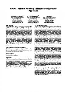
Fig. 4. SVM 2D classification map example for normal operation of OR1(red region) and OR2 (blue region). Green region is common to both OR1 and OR2

Training an SVM on a feature set implies a nonlinear mapping of the inputs into a higher dimensional feature space where classification of input data is possible. Figure 4 illustrates a 2D projection of the features for OR1 and OR2 that shows the regions for normal operation in the tested operating regimes. The normal operation of OR1 is displayed in red, The normal operation of OR2 is displayed in blue and the common normal region for both regimes is displayed in green.

Fig. 2. Health indicator result using SOM machine on RB1 (blue line) and RB2 (green line) data

Fig. 5.

Fig. 3. Health indicator result using a SVM on RB1 (blue line) and RB2 (green line) data

C. Tracking Multi-condition Degradation of Roller Bearing The degradation of a bearing may be observed in all available operation regimes. Using a healthy operation regime may nevertheless extend the life of a bearing. The degradation

SVM testing: heath indicator and contribution factors

By simultaneously monitoring the roller bearing degradation for multiple operating modes (either by using the SVM or the SOM) one can track the overall behavior and health of the bearing. This is done by computing the health indicator in every tested data point together with the contribution factors of the selected feature set described in the Section 3. Figure 5 displays a sample test point with its associated feature contributions in comparison to the training feature set. The changes seen in the features (see Figure 6) give indication about the root causes of bearing observations and can support field engineers in identifying and explaining unknown roller bearing faults.

Fig. 6.

SVM testing: contribution factors of selected features

IV. D ISCUSSION OF RESULTS The learned SOM and SVM models have similar performance on the test cases selected in this paper. They both have predictive power and track incipient faults. The models have been trained with a small number of input features (four) that have been heuristically defined by human experts. Small input dimensionality was required given the relatively small data sets used in the experiments. We have varied the input features and found predictive capabilities in other input subspaces as well. In preliminary investigations, higher frequency input features appear to result in a health indicator measure that can predict faults earlier than the low frequency features used in Section III, but which also give a higher false alarm rate. This aspect is presently under investigation. The SVM approach can be generalized to employ a learning procedure that prunes features or penalizes the criterion if too many weights are non zero, to drive towards a sparse weight vector, and therefore do an automatic feature selection. This is the typical approach in the literature. Feature pruning is desirable, as it typically leads to an increase in the generalization ability of the classifier (and thus its accuracy) and possibly improves convergence of the trained model. Recent literature suggests joint feature selection and SVM learning. For example [20] proposes a convex optimization for the joint learning approach to prevent the loss of information relevant to the classification task. Such approaches, however, require very large amounts of training data. As shown, multi-modal analysis of defects can improve the early prediction performance of incipient faults/degradation by simultaneously looking at all investigated operating regimes. Moreover, the analysis of the feature contribution offers enhanced capabilities to field engineers in understanding the root causes of bearing faults and supporting them in the decision making process. V. C ONCLUSION Timely detection of roller bearing defects is key to efficient service management, cost saving strategies and extended utilization, especially in hard accessible places as off-shore wind

turbines. By using a statistical models for diagnosis, one can observe and detect faulty operation, identify known defects and monitor the degradation level of bearings. Furthermore, one can correlate ongoing observations to the change in time of the investigated features. The approach discussed in this paper describes a workflow for monitoring of roller bearing degradation under different operating regimes. Both SOM and one-class SVM have been applied to detect bearing degradation over time. The models have been tested on multiple bearings of the same type. The results show that both SOM and SVM can effectively monitor the bearing degradation and that the generated health indicator can be well correlated with the engineering maintenance log. By processing daily measurements and taking into consideration historical records, the trained models are able to predict incipient bearing faults, save time and cost of repairs and increase availability. The generality of the health indicator needs to be further investigated with data collected from a large number of bearings. One of the challenges is how to identify the normality baselines. The automatic adaptation to new operating regimes needs to be addressed in future research. Future work will address automatic selection of features and automatic adaptation to new operating regimes. R EFERENCES [1] S. Abbasiona, A. Rafsanjania, A. Farshidianfarb, N. Iranic, Rolling element bearings multi-fault classification based on the wavelet denoising and support vector machine, Mechanical Systems and Signal Processing, 21(7):2933–2945, 2007. [2] D.Dahl, D.Sosnowski, D.Schlegel, R.J.Kerkman, M.Pennings, Field Experience Identifying Electrically Induced Bearing Failures, Pulp and Paper Industry Technical Conference, 2007. [3] S. J. Lacey, An Overview of Bearing Vibration Analysis, IEEE PES Transmission and Distribution Conference and Exposition Latin America, Venezuela, 2006. [4] Irahis Rodrguez, Roberto Alves, Bearing Damage Detection of the Induction Motors using Current Analysis, Maintenance & Asset Management, 23(6), 2008. [5] Tatsunobu Momono and Banda Noda, Sound and Vibration in Rolling Bearings, Motion & Control, 6, 1999. [6] R.R. Schoen, T.G. Habetler, F. Kamran, R.G. Bartfield, Motor bearing damage detection using stator current monitoring, IEEE Transactions on Industry Applications, 31(6):1274–1279, 1995. [7] Achmad Widodo, Eric Y. Kim, Jong-Duk Son, Bo-Suk Yang, Andy C.C. Tan, Dong-Sik Gu, Byeong-Keun Choi, Joseph Mathew, Fault diagnosis of low speed bearing based on relevance vector machine and support vector machine, Expert Systems with Applications, 36(3):7252–7261, 2009. [8] Yu Yang, Dejie Yu, Junsheng Cheng, A fault diagnosis approach for roller bearing based on IMF envelope spectrum and SVM, Measurement, 40(9):943–950, 2007. [9] M. Zacksenhouse, S. Braun, M. Feldman, Toward helicopter gearbox diagnostics from a small number of examples, Mechanical Systems and Signal Processing, 14(4):523–543, 2000. [10] Thomas Cormen, Charles Leiserson, Ronald Rivest, Clifford Stein, Introduction to Algorithms, 2002. [11] L. Liao, R. Pavel, Machine Anomaly Detection and Diagnosis Incorporating Operational Data Incorporating Operational Data Applied to Feed Axis Health Monitoring, ASME 2011 International Manufacturing Science and Engineering Conference, 2011. [12] Richard Duda, Peter Hart, David Stork, Pattern Classification, 2nd ed., Wiley–Interscience, 2000. [13] T. Kohonen, The self-organizing map, Proceeding of the IEEE,78(9):1464–1480, 1990.

[14] L. Liao, H. Wang, J. Lee, Bearing Health Assessment and Fault Diagnosis Using the Method of Self-Organizing Map, 61st Meeting of the Society for Machinery Failure Prevention Technology, 2007. [15] V. Vapnik, Statistical Learning Theory, New York: Wiley, pp. 128–136, 1998. [16] Guang-Ming Xian, Bi-Qing Zeng, An intelligent fault diagnosis method based on wavelet packer analysis, Expert Systems with Applications, 36: 1213112136, 2009. [17] Ha Quang Minh, Partha Niyogi, Yuan Yao, Mercers Theorem, Feature Maps, and Smoothing, Computational Learning Theory - COLT , pp. 154–168, 2006. [18] Chih-Chung Chang and Chih-Jen Lin, LIBSVM : a library for support vector machines, ACM Transactions on Intelligent Systems and Technology, 2(3):1–27, 2011. [19] Yihua Zhou, A Relevance Feedback Algorithm Based on SVM Model’s Dynamic Adjusting for Image Retrieval, Computational Intelligence and Security Workshops, pp: 287–290, 2007. [20] Minh Hoai Nguyen, Fernando de la Torre, Optimal feature selection for support vector machines, Pattern Recognition, 43(3):584-591, 2010.