Proceedings of the International MultiConference of Engineers and Computer Scientists 2010 Vol III, IMECS 2010, March 17 - 19, 2010, Hong Kong
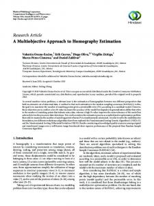
A Multi-objective Approach for Multi-commodity Location within Distribution Network Design Problem H. Afshari, M. Amin-Nayeri, A. A. Jaafari Abstract— This paper presents a multi-objective mixed integer programming formulation for location within network distribution problem. Objectives are to minimize total cost including establishment and transportation cost and to maximize customer satisfaction. The problem describes two location layers in single period. We determine the volume of the inventory in both stocks and middle warehouses. Index Terms— Location, Multi commodity, Multi objective, Network design.
I. INTRODUCTION Supply chain management (SCM) is the process of planning, implementing and controlling the operations of the supply chain in an efficient way. SCM spans all movements and storage of raw materials, work-in-process inventory, and finished goods from the point-of-origin to the point-of-consumption (Council of Supply Chain Management Professionals 2007, Simchi-Levi et al. 2004). There are more works in literature considering concepts of SCM in variant areas that we state some of them as follows. Altiparmak et al. (2006) developed a multi-objective genetic algorithm (MOGA) to find a set of optimal pareto solution for Supply chain network (SCN) design. Thanh et al. (2008) proposed a mixed integer programming (MIP) formulation to design and plan a production –distribution system along the supply chain. Pujari et al. (2008) presented an integrated approach for incorporation of location, production, inventory and transportation issues within a supply chain. Shu and Karimi (2009) developed two heuristic algorithms for considering concept of safety stock in supply chain networks. Kaminsky and Kaya (2008) proposed effective heuristics for inventory positioning in supply chain networks involving several centrally managed production facilities and external suppliers. Monthatipkul and Yenradee (2008) introduced an MIP model to find an optimal inventory/distribution plan (IDP) control system for a one-warehouse/multi-retailer supply chain system. Chauhan et al. (2009) designed a heuristic for Multi-commodity supply network planning and a branch and price for large-sized problems. Khouja formulated a three-stage supply chain model and investigate effect of change from two-stage from three-stage in cost reduction. Seliaman and Ahmad consider three-stage supply chain with stochastic demand to optimize inventory decision. Santoso et al. (2005) proposes a stochastic programming formulation for supply chain under uncertain environment. Newly, a single vendor and multiple retailers H. Afshari, M. Aminnayeri, A. A. Jaafari are with the Department of Industrial Engineering, Amirkabir University, Tehran, Iran (e-mail: e-mail:
[email protected])
ISBN: 978-988-18210-5-8 ISSN: 2078-0958 (Print); ISSN: 2078-0966 (Online)
supply chain retailers is modeled (Darwish and Odah, to be published). For more detailed study, Gunasekaran and Ngai (2009) and Minner (2003) can be useful. Facility location is and has been a well established research area within Operations Research (OR). Numerous papers and books are witnesses of this fact. The development of SCM started independently of OR and only step by step did OR enter into SCM. As a consequence, facility location models have been gradually proposed within the supply chain context (including reverse logistics), thus opening an extremely interesting and fruitful application domain (Melo et al. 2009). Here, some previous researches worked on location within supply chain, are described. Gebennini presented a model for location-allocation problem to optimize safety stocks and customer service level. Snyder et al. (2007) proposed a stochastic version of the location model with risk pooling (LMRP) that include location, inventory, and allocation decisions under uncertainty. Syam (2002) extend facility location problem considering several concepts of logistic as holding, ordering, and transportation costs. He used two lagrangian relaxation and a simulated annealing (SA) based heuristics algorithm for comparing experimental results. Thanh et al. (2008) consider facility location problem in supply chain within planning horizon. Melo et al. (2009) reviewed facility location problem in a well-organized way that it can be useful for being depth in this area. In this paper, we present a multi-objective mixed integer programming formulation for location within network distribution problem. Objectives are to minimize total cost including establishment and transportation cost and to maximize customer satisfaction. The problem describes two location layers in single period. We determine the volume of the inventory in both stocks and middle warehouses. The remainders of paper are as follows. Model description is stated in section II. In, Section III, mathematical model is formulated, computational results are indicated in section IV and conclusions are discussed in section V. II. MODEL DESCRIPTION Components of supply chain such as are illustrated in Figure 1 are introduced. Central warehouses: the main stocks of supply chain that demands are supplied here. There are two potential location for central warehouses, capital of country and south port. Regional warehouses: stocks between central warehouses and customers that demands are distributed here. There are 8 potential locations for regional warehouses that they are in the capital of provinces.
IMECS 2010
Proceedings of the International MultiConference of Engineers and Computer Scientists 2010 Vol III, IMECS 2010, March 17 - 19, 2010, Hong Kong Customers: there are 28 customers that are located in the cities of the provinces. Goods: Five types of commodities can be supplied for the customers demanding five families of cars. Fig 1. Components of supply chain Customers Regional Warehouses
Distance between regional warehouse 𝑗 and customer 𝑖, Distance between regional warehouse 𝑗 and central warehouse 𝑘, Capacity of central warehouse 𝑘 for commodity 𝑡, Coefficient of total cost in objective function, Cost of installation central warehouse 𝑘, Minimum level of customer satisfaction 𝑖 for commodity𝑡. Cost of installation regional warehouse 𝑗,
𝑑𝑖𝑗 ′ 𝑑𝑗𝑘
𝑒𝑘𝑡 𝑃 𝑞𝑘 𝑠𝑖𝑡 𝑤𝑗
D. Mathematical Model 𝑜
Central Warehouses
𝑚
𝑛
𝑀𝑖𝑛 𝑍1 = 𝑃 . . .
}
8
. . .
𝑜
}
28
𝑙
𝑐. 𝑑𝑖𝑗 𝑎𝑖𝑡 𝑥𝑖𝑗𝑡 𝑡=1 𝑗 =1 𝑖=1 𝑚
𝑡=1 𝑘=1 𝑗 =1
1 𝑀𝑎𝑥 𝑍2 = 1 − 𝑃 𝑛. 𝑜 𝑜
𝑚
𝑙
′ 𝑐. 𝑑𝑗𝑘 𝑎𝑖𝑡 𝑥𝑖𝑗𝑡 + 𝑃
+𝑃
𝑛
𝑜
𝑛
𝑤𝑗 𝑢𝑗 + 𝑃 𝑗 =1 𝑚
𝑞𝑘 𝑣𝑘 𝑘=1
𝑥𝑖𝑗𝑡 𝑡=1 𝑖=1 𝑗 =1
𝑥𝑖𝑗𝑡 ≤ 𝑛. 𝑜. 𝑢𝑗
∀𝑗
1
𝑦𝑗𝑘𝑡 ≤ 𝑚. 𝑜. 𝑣𝑘
∀𝑘
2
𝑎𝑖𝑡 𝑥𝑖𝑗𝑡 ≤ 𝑏𝑗𝑡
∀𝑗, 𝑡
3
𝑏𝑗𝑡 𝑦𝑗𝑘𝑡 ≤ 𝑒𝑘𝑡
∀𝑘, 𝑡
4
𝑥𝑖𝑗𝑡 ≥ 𝑠𝑖𝑡
∀𝑖, 𝑡
5
∀𝑗, 𝑡
6
𝑡=1 𝑖=1 𝑜 𝑚
Assumptions of problem are as follows: There are two potential central warehouses that at least one of them should be located, There are limited capacities for both central and regional warehouses. Transportation cost per unit is as a coefficient of distance between central and regional warehouses and between regional warehouses and customers. There is a minimum level of customer satisfaction. There are two objectives for supply chain, minimizing total cost including establishment and transportation cost and maximizing customer satisfaction.
𝑡=1 𝑗 =1 𝑛
𝑖=1 𝑚
𝑗 =1 𝑚
𝑗 =1 𝑙
𝑛
𝑏𝑗𝑡 𝑦𝑗𝑘𝑡 ≤ 𝑘=
𝑢𝑗 , 𝑣𝑘 𝜖 0,1
𝑎𝑖𝑡 𝑥𝑖𝑗𝑡 𝑖=1
III. MODEL FORMULATION A. Sets and indices 𝐿 Sets of central warehouses 𝐿 = 𝑙, 𝑘𝜖𝐿 , 𝑀 Sets of regional warehouses 𝑀 = 𝑚, 𝑗𝜖𝑀 , 𝑁 Sets of customers 𝑁 = 𝑛, 𝑖𝜖𝑁 , 𝑂 Sets of good types 𝑂 = 𝑜, 𝑡𝜖𝑂 . B. Variables 1, If the potential point of 𝑘 for 𝑣𝑘 = central warehouses is located, 0, Otherwise, 1, If the potential point of 𝑗 for 𝑢𝑗 = regional warehouses is located, 0, Otherwise, Percentage of demand customer 𝑖 for commodity 𝑡 𝑥𝑖𝑗𝑡 that is supplied by regional warehouse𝑗, Percentage of demand regional warehouse 𝑗 for 𝑦𝑗𝑘𝑡 commodity 𝑡 that is supplied by central warehouse𝑘. C. Parameters Demand of customer 𝑖 for commodity𝑡, 𝑎𝑖𝑡 Capacity of regional warehouse 𝑗 for commodity 𝑡, 𝑏𝑗𝑡 Cost of transportation per unit, 𝑐
ISBN: 978-988-18210-5-8 ISSN: 2078-0958 (Print); ISSN: 2078-0966 (Online)
First objective 𝑍1 , is summation of: Transportation cost between central and regional 𝑛 warehouses, 𝑜𝑡=1 𝑚 𝑗 =1 𝑖=1 𝑐. 𝑑𝑖𝑗 𝑎𝑖𝑡 𝑥𝑖𝑗𝑡 , Transportation cost between regional warehouses ′ and customer, 𝑜𝑡=1 𝑙𝑘=1 𝑚 𝑗 =1 𝑐. 𝑑𝑗𝑘 𝑎𝑖𝑡 𝑥𝑖𝑗𝑡 , Installation cost for central warehouses, 𝑚 𝑤 𝑢 and 𝑗 =1 𝑗 𝑗 Installation cost for regional warehouses, 𝑙𝑘=1 𝑞𝑘 𝑣𝑘 , that is multiplied by weighted coefficient 𝑃. Second objective, 𝑍2 , is the summation of the level of the customer satisfaction that is multiplied by 1 − 𝑃 . Constraints (1) and (2) states if regional warehouse 𝑗 or central warehouse 𝑘 satisfy the demand, it has been installed. Constraints (3) and (4) show capacity restriction for each regional warehouse. Constraint (5) implies that there is a minimum level of customer satisfaction 𝑖 for commodity 𝑡. Constraint (6) considers that amount of supply should be greater than amount of demand.
IMECS 2010
Proceedings of the International MultiConference of Engineers and Computer Scientists 2010 Vol III, IMECS 2010, March 17 - 19, 2010, Hong Kong
B. Experimental results As designed and considered in the model, this can be applied for many real cases and because of the multi-objective nature of the model, a weighting mechanism was used to unite all objective functions. So the model is solved with different weights and this could help the model users to select proper strategies. For example, the fig 1 demonstrates the costs of the distribution system in different customer satisfaction values at 𝑠𝑖𝑡 =0.1. This figure can be showed at different 𝑠𝑖𝑡 values. These figures could be useful to balance between cost and satisfaction. Table 1 Shows the Computational results for different P values at different 𝑠𝑖𝑡 . In bi-objective problems, it’s easier to select optimal or near optimal solutions but not still mistake proof. Proper tuning of parameters is essentially important to guide optimal solution. fig 2 shows that how much it could be critical to adjust parameters and the necessity of wisely solution selection after parameter tuning. A method to coup with these difficulties is defining a new function which is the percentage summation of satisfaction and total costs divided by maximum cost in each p value. The new function shows how to get desired aim in minimum costs and minimum customer dissatisfaction. Fig 3 demonstrates
ISBN: 978-988-18210-5-8 ISSN: 2078-0958 (Print); ISSN: 2078-0966 (Online)
Fig 1. Total Costs vs. Satisfaction Level at 𝑠𝑖𝑡 =0.1
Customer Satisfaction
1 0.8 0.6 0.4 0.2 0 1
2E+09
4E+09
6E+09
8E+09
1E+10
Total Costs Fig 2. Total Costs vs. Min Service Level at 𝑃=0.1 to 1
Minimum Service Level
A. Case study This model is presented for a practical case in Automotive Part Distribution Corporation. So the new model was extended to be replaced with previous one which was implemented for 40 years. Former distribution system contained one central warehouse and the commodities were directly transshipped to customers. This outmoded distribution system was faced with new aggravating problems and management board decided to apply new distribution system. Many choices were suggested to improve critical strategic indexes such as market share, customer satisfaction, demand response time, transportation costs and inventory costs including warehousing costs in central warehouse and backordering costs. To improve these indexes, new distribution system was applied to be adjacent to customer zone and agile response to customer needs and to increase market share. Therefore all of the customers were categorized to particular zones in order to create nominated areas for establishing regional warehouses. Finally 8 potential zones were to be nominated for selection as regional warehouses and it was time to apply customer demands of different commodities, distances of nominated areas from central warehouses and customers and other constraint as described in model. Another main contribution which was suggested to coup with the problems was testing whether establishing new central warehouse would be useful and reasonable or not. For testing this, considerations were included in the model to be concluded the suggestion accuracy and sufficiency. The main idea aspired this suggestion was the volume of imports of spare parts from foreign countries which are delivered in one of south ports. The parameters and constants which are used in this model are gained based on real data of system and eagerly chased to see the model outcomes. So for comparison, some criteria are considered to assess the efficiency of model.
new function values vs. different 𝑠𝑖𝑡 .
1
0.8 0.6 0.4 0.2
p=1 p=0.9 p=0.7 p=0.5 p=0.3 p=0.1
0
Total Costs
Fig 3. New Function Value vs. Min Service Level 1.00
New Function Value
IV. COMPUTATIONAL RESULTS
0.95
p=0.1
0.90 0.85
p=0.3
0.80
p=0.5
0.75 p=0.7
0.70 0.65
p=0.9
0
1
2
3
4
5
6
7
8
9
10
Minimum Service Level
According to fig 3, first it must be decided that what could be the minimum service level then finding the minimum function value in relevant service level and the proper coefficient in total objective value will be obtained. Table 2 demonstrates calculation results of model for mentioned case studied at 𝑠𝑖𝑡 =0.6 and P=0.5. Table 2. Results of designed model at 𝑃=0.5 & 𝑠𝑖𝑡 =0.6
Variable Title 𝒁𝟏 𝒁𝟐
V(1,2) U(1,2,3,4,5,6,7,8)
Value 4.56E+09 82% (1,1) (1,0,1,1,0,1,0,1)
IMECS 2010
Proceedings of the International MultiConference of Engineers and Computer Scientists 2010 Vol III, IMECS 2010, March 17 - 19, 2010, Hong Kong [6]
V. CONCLUSION Extension of supply chain concept to real problems has caused the issue to be more interesting. New problems include more variable and parameters. Also it is expected that the designed models fulfill more objectives. This paper is an embodiment of this issue. This model is presented for multi-objective multi commodity location problems. Nonconformity between objective functions is a concern and just weighting couldn’t be sufficient to support the aims. Therefore some contribution is needed. In this paper a mix integer model is presented and it is solved with LINGO software. According to acquisition of model parameters from real case, the model outcomes were used for decision making. The results showed to be practical and useful because of great similarities between the model and the studies case and ensured that this model can be applied for other cases. Finally, the future extensions to the model could be considering the multi-stage situation. Another contribution would be adding components to fulfill demand uncertainties.
[7]
REFERENCES
[16]
[1]
[2]
[3] [4]
[5]
Altiparmak F, Gen M, Lin L, Paksoy T, A genetic algorithm approach for multi-objective optimization of supply chain networks, Computers & Industrial Engineering 51 (2006) 196–215. Chauhan S. S, Frayret J-M, LeBel L, Multi-commodity supply network planning in the forest supply chain, European Journal of Operational Research 196 (2009) 688–696. Council of Supply Chain Management Professionals, , 2007. D. Simchi-Levi, P. Kaminsky, E. Simchi-Levi, Managing the Supply Chain: The Definitive Guide for the Business Professional, McGraw-Hill, New York, 2004. Darwish M. A, Odah O. M, Vendor Managed Inventory Model for Single-Vendor Multi-Retailer Supply Chains, To be published in European Journal of Operational Research.
ISBN: 978-988-18210-5-8 ISSN: 2078-0958 (Print); ISSN: 2078-0966 (Online)
[8]
[9]
[10]
[11]
[12]
[13]
[14]
[15]
[17]
[18]
[19]
Gebennini E, Gamberini R, Manzini R, An integrated production–distribution model for the dynamic location and allocation problem with safety stock optimization, International Journal of Production Economics 122(2009)286–304. Gunasekaran A, Ngai E. W.T, Modeling and analysis of build-to-order supply chains, European Journal of Operational Research 195 (2009) 319–334. Kaminsky P, Kaya O, Inventory positioning, scheduling and lead-time quotation in supply chains, International Journal of Production Economics 114 (2008) 276–293. Khouja M, Optimizing inventory decisions in a multi-stage multi-customer supply chain, Transportation Research Part E 39 (2003) 193–208. Melo M.T, Nickel S, Saldanha-da-Gama F, Facility location and supply chain management – A review, European Journal of Operational Research 196 (2009) 401–412. Minner S, Multiple-supplier inventory models in supply chain management: A review, International Journal of Production Economics 81–82 (2003) 265–279. Monthatipkul C, Yenradee P, Inventory/distribution control system in a one-warehouse/multi-retailer supply chain, International Journal of Production Economics, 114 (2008) 119–133. Pujari N. A, Hale T. S, Huq F, A continuous approximation procedure for determining inventory distribution schemas within supply chains, European Journal of Operational Research 186 (2008) 405–422. Santoso T, Ahmed S, Goetschalckx M, Shapiro A, A stochastic programming approach for supply chain network design under uncertainty, European Journal of Operational Research 167 (2005) 96–115. Seliaman M.E, Ahmad A A, Optimizing inventory decisions in a multi-stage supply chain under stochastic demands, Applied Mathematics and Computation 206 (2008) 538–542. Shu j, Karimi I. A, Efficient heuristics for inventory placement in acyclic networks, Computers & Operations Research 36 (2009) 2899-2904. Snyder L. V, Daskin M. S, Teo C-T, The stochastic location model with risk pooling, European Journal of Operational Research 179 (2007) 1221–1238. Syam S. S, A model and methodologies for the location problem with logistical components, Computers & Operations Research 29 (2002) 1173-1193. Thanh P. N, Bostel N, Pe´ton O, A dynamic model for facility location in the design of complex supply chains, International Journal of Production Economics 113 (2008) 678–693.
IMECS 2010
Proceedings of the International MultiConference of Engineers and Computer Scientists 2010 Vol III, IMECS 2010, March 17 - 19, 2010, Hong Kong
0.1 0.2 0.3 0.4 𝑃
0.5 0.6 0.7 0.8 0.9
Table 1. Computational results for different 𝑃 𝑆𝑖𝑡 0.4 0.5 0.6 0.7
0.1
0.2
0.3
0.8
0.9
1
𝑍1
3.33E+09
5.17E+09
5.93E+09
6.05E+09
6.21E+09
6.25E+09
6.33E+09
6.65E+09
6.65E+09
1.03E+10
𝑍2
0.8
0.94
0.98
0.99
0.99
0.99
0.99
1
1
1 1.03E+10
𝑍1
1.67E+09
2.85E+09
4.32E+09
5.31E+09
5.45E+09
5.99E+09
6.12E+09
6.25E+09
6.60E+09
𝑍2
0.51
0.71
0.87
0.95
0.95
0.98
0.99
0.99
1
1
𝑍1
1.46E+09
2.72E+09
2.91E+09
4.16E+09
4.66E+09
5.45E+09
5.61E+09
6.14E+09
6.32E+09
1.03E+10
𝑍2
0.44
0.69
0.67
0.83
0.87
0.95
0.95
0.98
0.99
1
𝑍1
1.07E+09
2.03E+09
2.85E+09
3.42E+09
4.28E+09
4.66E+09
5.43E+09
6.01E+09
6.25E+09
1.03E+10
𝑍2
0.27
0.5
0.66
0.71
0.82
0.84
0.93
0.97
0.98
1
𝑍1
1.06E+09
1.75E+09
2.39E+09
2.95E+09
4.05E+09
4.56E+09
5.32E+09
5.94E+09
6.20E+09
1.03E+10
𝑍2
0.26
0.37
0.47
0.57
0.77
0.82
0.91
0.96
0.97
1
𝑍1
1.06E+09
1.75E+09
2.37E+09
2.94E+09
3.83E+09
4.43E+09
5.15E+09
5.69E+09
6.16E+09
1.03E+10
𝑍2
0.26
0.37
0.46
0.57
0.69
0.78
0.86
0.91
0.96
1
𝑍1
1.03E+09
1.74E+09
2.36E+09
2.92E+09
3.80E+09
4.21E+09
4.98E+09
5.63E+09
6.12E+09
1.03E+10
𝑍2
0.22
0.36
0.46
0.55
0.68
0.68
0.8
0.89
0.95
1
𝑍1
1.03E+09
1.73E+09
2.35E+09
2.91E+09
3.73E+09
4.20E+09
4.96E+09
5.61E+09
6.10E+09
1.03E+10
𝑍2
0.21
0.33
0.44
0.55
0.62
0.67
0.79
0.88
0.94
1
𝑍1
1.03E+09
1.72E+09
2.32E+09
2.89E+09
3.71E+09
4.18E+09
4.93E+09
5.59E+09
6.09E+09
1.03E+10
𝑍2
0.21
0.32
0.39
0.5
0.58
0.64
0.75
0.85
0.93
1
ISBN: 978-988-18210-5-8 ISSN: 2078-0958 (Print); ISSN: 2078-0966 (Online)
IMECS 2010