A Multi-objective Differential Evolution Algorithm for Robot Inverse

SSRGInternational International Journal Journal of of Computer -volume 3 Issue 11 -November 2016 SSRG Computer Science Scienceand andEngineering Engineering(SSRG-IJCSE) (SSRG-IJCSE) – volume 3 Issue 10–October2016

A Multi-objective Differential Evolution Algorithm for Robot Inverse Kinematics Enrique Rodriguez#1, Baidya Nath Saha*2, Jesús Romero-Hdz#3, David Ortega*4 #1

Universidad Autónoma de Nuevo León, San Nicolás de los Garza, México *2 Centro de Investigación en Matemáticas(CIMAT), Monterrey, México #3,*4 Centro de Ingeniería y Desarrollo Industrial(CIDESI), Monterrey, México [email protected], [email protected]

{3jaromero, 4Ortega.a}@posgrado.cidesi.edu.mx

Abstract — This paper presents the robot inverse kinematics solution for four Degrees of Freedom (DOF) through Differential Evolution (DE) algorithm. DE can handle real numbers (float, double) which leads more powerful than Genetic Algorithm (GA). We propose a multi-objective fitness function that makes an attempt to minimize the positional error and maximum angular displacement of the robot joints. Maximum angular displacement based fitness function adopt the constraints on different unrealistic rotational movement of the manipulator. We employ an equitable treatment of both fitness functions while maximizing these two over generations that iteratively selects the optimal weights of these two fitness functions automatically. Trigonometric mutation and binomial crossover improve the performance of the conventional DE technique. We compared the results of proposed multi-objective DE with GA and Algebraic Method (AM). Proposed multi-objective DE algorithm obtains less positional error than conventional DE, GA and AM while meeting the rotational constraints of the manipulator’s joints. Keywords— Inverse Kinematic, Differential Evolution, Multi-objective optimization, Genetic Algorithm, Robot manipulator with four degrees of freedom. I. INTRODUCTION Robot inverse kinematics is a topic largely addressed in robotic research for many years. Advancement of robotics technology are enlarging it areas of application and hence robots are now often used in day-to-day activities of many fields of industry, science, and medicine. This elevates the inverse kinematics problem to the upfront of the robotic research. The inverse kinematics problem is to find the angular position of the robot joints which can achieve some expected position and orientation of the end effector that allows the robot to execute the required task. The angular position of the robot joints is required to transform a motion so that the robot can perform some given tasks such as peg-hole insertion, parts mating and manufacturing assembly operation which are very common in day-to-day industry operation [1].

ISSN: 2348 – 8387

Robot kinematics problem can be categorized into two classes: forward kinematics problem in which position and orientation of the end effector can be directly computed from the angular position of the robot joints using Denavit-Hartenberg (DH) method and the inverse kinematics problem which is defined above. The inverse kinematics problem is quite complex because it deals with solving a system of underdetermined nonlinear equations. As a result, this is not always possible to find a closed-form solution. Due to the underdetermined nature of the problem, sometimes multiple solutions may exist, however, none of them may not be admissible for the existing kinematic structure of the robot. In some cases, no solution at all may exist, i.e., robot cannot achieve the desired position and orientation of the end effector because it is very difficult to find the suitable constraints for solving the underdetermined system of non-linear equations. Different solution techniques for this problem can be categorized into two major classes: closed-form analytical and numerical methods. Closed-form solutions are faster than the numerical solutions and it can identify all possible solutions, but these techniques are dependent on robot kinematic structure and it is not possible to obtain for different robot kinematic structures such as Crustcrawler AX-18 Smart Robotic Arm [2]. In contrast, numerical solutions are more general because they are not dependent of the robot structure. However, numerical methods are slower because they normally first guess an initial solution and then find the final solution in an iterative manner and they converge into local optima. The quality of the solution depends on the set of starting values. In addition, when the numerical methods fail to converge, they cannot obtain the solution even if the solution of the inverse kinematics problem exists. In this research we aim at determining the solution of inverse kinematics problem for Crustcrawler AX18 Smart Robotic Arm which has four degrees of freedom and a gripper. This kind of robot manipulator are widely used in different industrial applications such as peg-hole insertion tasks, complex manipulations, obstacle avoidance and assistance tasks like serving drink to the users [3]. Though there are few closed form solutions using algebraic method

www.internationaljournalssrg.org

Page 71 1

SSRGInternational International Journal Journal of -volume 3 Issue 11 -November 2016 SSRG of Computer Computer Science Scienceand andEngineering Engineering(SSRG-IJCSE) (SSRG-IJCSE) – volume 3 Issue 10–October2016

available in literature [1], [4], [5] for inverse kinematics of Crustcrawler AX-18 robot manipulator, however it does not always guarantee to provide the admissible solutions. To demonstrate this phenomenon, we conducted a simulation experiment using P. Corke’s matlab toolbox [6] with a four link robot manipulator with four degrees of freedom. The length of the links are equal to the length of the links of the Crustcrawler AX-18 robot manipulator [2] used in this experiment that are provided in Table 1.

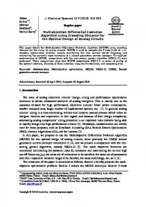
Fig. 1 Two different configurations of the robot achieving the same target position, px = 10, py =10, pz =10.

Fig. 1 shows the results of two robot configurations which can achieve the final target location px = 10, py =10, pz =10. Fig. 1 is developed using P. Corke’s matlab toolbox. We used different evolution algorithm to find the robot inverse kinematics solutions under two different conditions: without restrictions and with restrictions. The restriction includes the real constraint on angular displacement of the servomotor of the Crustcrawler AX-18 robot manipulator based on the capacity of the servomotor [2]. The restrictions are:

1   150 ,150 ,  2   60 ,240 , 3   150 ,150 ,  4   150 ,150  . The solutions found without restrictions are θ1= -135o, θ2= -123.27o, θ3= 188.83o, and θ4= 134.84o and with restrictions are θ1= 45o, θ2= 72.42o, θ3= -2.29o, and θ4= -133.6o. The results show that the robot configuration without restrictions violate the constraints on θ2 and θ3. However, we found a viable solution with restrictions. This experiment shows that multiple solutions exist in robot inverse kinematics problem due to underdetermined nature of the linear systems (we have three linear equations for solving four degrees of freedom of the robot joints). Finding such viable solutions require an exhaustive search which is not always practically feasible for higher dimensions. Existing numerical methods on evolutionary algorithms, to name a few genetic algorithm [7], [8] and differential evolution [9], [10] provide solutions for the problems of exhaustive search with acceptable accuracy. In practice, usually manually designed look-up tables based approximate

ISSN: 2348 – 8387

inverse kinematics based solutions are used for controlling a robotic manipulator [11].

Existing research efforts based on evolutionally algorithms towards robot inverse kinematics mainly deal with minimizing the positional error. However, it is found that even the robot can achieve the target position with minimal position error, the solutions are not admissible solutions (the required robot configuration to achieve the target position is many times practically not feasible) due to the limitations of the servomotor to achieve very high angular displacement as shown in Fig. 1. However, success of differential evolutions for its faster convergence and more accurate solutions over genetic algorithm (DE can tackle real and floating point numbers which is required for robot joint angles) has attracted to develop a multi-objective differential evolution algorithm for robot inverse kinematics problem. Unlike the existing researches, along with minimizing positional error, we try to minimize the maximum of the angular displacement of robot joints which naturally restrains on robot angular displacement and avoids to find the robot configuration with high angular displacement of the joints and hence assists in finding admissible solutions. Thus the proposed multi-objective differential evolution algorithm offers a practically viable solution for robot inverse kinematics problem through achieving the target position with minimal positional error and satisfying the angular constraints of the robot joints. This research offers the following technical contributions. Firstly, we propose a multi-objective differential evolution algorithm for robot inverse kinematics problem. Secondly, we proposed two fitness functions: a) the first one minimizes the final positional error of the robot and (b) the second one minimizes the maximum angular displacement of the robot angular joints. The second fitness function restricts the rotational displacement of the angular joints of the robot while the first one attempts to arrive the end effector of the robot to the target position with minimal positional error. Thirdly, we employ an unbiased treatment of both fitness functions that selects the optimal weights between these two functions iteratively over the generations. Fourthly, we exploited binomial crossover and trigonometric mutation for differential evolution approach that accelerates the convergence of the differential evolution algorithm. We implemented the multi-objective differential algorithm on Crustcrawler AX-18 robot manipulator [2] with four degrees of freedom. We also conducted the sensitivity analysis of the proposed algorithm. Experimental results demonstrate that proposed multi-objective differential evolution algorithm achieves less positional error and satisfy the angular constraints of the robot manipulator than genetic algorithm and algebraic method. We also developed the forward kinematics for the Crustcrawler AX-18 robot manipulator using

www.internationaljournalssrg.org

Page 72 2

SSRGInternational InternationalJournal Journal of of Computer Computer Science -volume 3 Issue 11 -November 2016 SSRG Scienceand andEngineering Engineering(SSRG-IJCSE) (SSRG-IJCSE) – volume 3 Issue 10–October2016

the Denavit-Hartenberg(DH) method. We modified the inverse kinematics solutions of the algebraic method for Crustcrawler AX-18 robot manipulator. The organization of the remaining of the paper is as follows. Section II presents the literature review regarding the existing robot inverse kinematics solutions to algebraic method, genetic algorithm and differential evolution. Section III discusses the inverse kinematics problem formulation using algebraic, genetic and DE method. Section IV presents the proposed multi-objective differential evolution for robot inverse kinematics problems. Section V illustrates the experimental results and discussions. Section VI concludes the work. II. BRIEF LITERATURE REVIEW In this section, we present the existing solutions of robot inverse kinematics using three algorithms, Algebraic Method (AM), Genetic Algorithm (GA), and Differential Evolution (DE).

Raphson method to minimize the final error to zero of the genetic algorithm. F.Y.C. and S.P. [8] used a genetic algorithm to optimize the inverse kinematic for real-time trajectory planning manipulator. Using a new proposed crossover method called Dynamic Multilayered Chromosome Crossover (DMCC) they implemented the method for a planar manipulator of three degrees of freedom. The results indicated an improved of the number of iterations for the genetic algorithm. Zhen and Yan-Tao [13] proposed a multi population genetic algorithm (MPGA) in order to improve the global converge. Where the MPGA divides the whole population into several populations, then through artificial selection and an immigration operation forms a new population by selecting the best individuals from each category. The MPGA compared with the simple genetic algorithm (SGA) made the global solution more efficient and accelerated the converge speed.

A. Algebraic Method (AM) Sultan and Schwartz [4] presented a solution for the inverse kinematic of a 5 DOF robot arm which is practically a 4 DOF manipulator with a degree of freedom in the gripper. The inverse kinematic was obtained from the transformation matrix and the forward kinematic equations which resulted in two sets of possible solutions depending of the calculation of θ2 and θ3. The solution proposed can closely approximate desired points within 1 cm of the workspace boundaries. Ramirez and Toscano [1] proposed a closed-form solution to the inverse kinematic of a 5 DOF manipulator robot defining the existence conditions for all the possible solutions and the singular configurations were identified. The proposed method uses the desired position of the center of the gripper as well the direction of the gripper’s main axis. Mohammed and Sunar [12] studied the forward and inverse kinematic of a 4 DOF robotic arm. For the forward kinematic model, the problem was compared using the Denavit-Hartenberg convention and the product of exponentials, those two approaches showed an identical solution. In the solution for the inverse kinematic problem an algebraic method was implemented which made use of a fourth parameter besides the x, y, z desired point, called the end effector orientation.

C. Differential Evolution (DE) Gonzalez and Blanco [9] demonstrated that a memetic approach increases the converge of the differential evolution algorithm for the inverse kinematic problem. They introduced a local search mechanism called discarding. The results using a 3 DOF planar robot showed that the proposed method is able to solve the inverse kinematic accurately and in fewer generations than the conventional DE. Wang and Hao [10] studied the forward kinematic of a pneumatic parallel manipulator using genetic algorithm, particle swarm optimization and the differential evolution algorithms. The performance of the DE was quite better than the GA and PSO where the speed of the convergence of the DE was less than the other ones with a greater reliability to obtain the global optima for the forward kinematic. Nguyen and Ho Pham [14] proposed a hybrid differential evolution to train an adaptive MIMO neural network for the solution of inverse kinematic. The hybrid differential evolution algorithm applied to solve the inverse kinematic of a 3 DOF manipulator which is composed by the back-propagation algorithm and the DE algorithm proved a faster performance and better precision than the conventional backpropagation algorithm or the solely differential evolution algorithm.

B. Genetic Algorithm y(GA)

III.INVERSE KINEMATIC PROBLEM FORMULATION Given the current (initial) and the desired position of the end effector of the robot that is defined by the user, we formulate the robot inverse kinematic problem is to find the angular position of the end effector to reach the desired position with minimal positional error and the minimum rotational displacement between the current joint angles and the joint angles of the end effector.

Joey and David [7] introduced the genetic algorithms for solving the inverse kinematics problem for redundant robots using a single fitness function which integrates the error of the final end effector position and the desired position and an additional term based on the angular joint displacements from the initial position of the robot. The results showed a significantly large final positioning error. They proposed for a future work to employ the Newton-

ISSN: 2348 – 8387

www.internationaljournalssrg.org

Page 73 3

SSRGInternational International Journal Journal of of Computer -volume 3 Issue 11 -November 2016 SSRG Computer Science Scienceand andEngineering Engineering(SSRG-IJCSE) (SSRG-IJCSE) – volume 3 Issue 10–October2016

A. FORWARD KINEMATICS

For our robot manipulator, the value of d1= 4.36 cm, a1 = 6.75 cm, a2 = 17.23 cm, a3 = 6.3 cm, d2 = 2.0 cm and a4 = 11.7 cm. The DH parameters facilitates to obtain each homogeneous transformation i-1Ai for the four coordinate systems of the robot manipulator which is given by as follows.  cos  i   sin  i i 1 Ai   0   0 

 cos  i sin  i cos  i cos  i

sin  i sin  i  sin  i cos  i

sin  i 0

cos  i 0

ai cos  i   a i sin  i  di   1 

The transformation matrix that links the position and orientation of the end effector or TCP is given by 4  0R T5   i Ai 1   5 i 0  0

0

Fig. 2 Four DOF Crustcrawler AX-18 robot manipulator robot configuration

For a kinematic model, a robot manipulator can be considered as a chain of links attached by joints. We can determine the position and orientation of the end effector or TCP (Tool Center Point) given a set of geometrical characteristic of the robot and a base frame, and this analysis is called forward kinematics. We use the Denavit-Hartenberg(DH) convention for the representation of the robot forward kinematic model. The DH convention are described by four parameters (link length, link twist, joint distance and joint angle) as given below [15]. 1. Link length (ai) is the distance between zi-1 and zi axes along the xi axis, ai is the kinematic length of link (i). 2. Link twist (αi) is the required rotation of the zi-1 axis about the xi axis to become parallel to the zi axis. 3. Joint distance (di) is the distance between xi-1 and xi axes along the zi-1 axis. Joint distance is also called the link offset. 4. Joint angle (θi) is the required rotation of xi-1 axis about the zi-1 axis to become parallel to the xi axis. The robot studied in this paper has four revolute joints, the di has a fixed value and θi is the variable. After applying the DH convention on this robot manipulator as shown in Figure 1, the values of the four parameters (ai, αi, di and θi) are listed in the Table 1. Table 1. Denavit-Hartenberg Parameters Frame ai αi di θi O1 0 π/2 d1 θ1 O2 a1 0 0 θ2 O3 a2 0 0 θ3 O4 a3 π/2 0 θ4 O5 a4 0 d2 0

ISSN: 2348 – 8387

0

P5   1 

The 0R5 matrix is called the rotation matrix that describes the orientation of the frame O4 relative to the base frame and the vector 0P5 is the position of the center of the TCP frame. The matrix for the robot forward kinematics is presented where the notation used are ci=cosθi, si=sinθi, cij=cos(θi+θj), sij=sin(θi+θj), cijk=cos(θi+θj+θk) and sijk=sin(θi+θj +θk). After simplifying the 0P5 vector using the product and sum difference identities, we obtain the position of the end effector which is given by,

px  a4c1c234  d2c1s234  a1c1c2  a3c1c234  a2c1c23

p y  a4 s1c234  a1c2 s1  d 2 s1s234  a3 s1c234  a2 s1c23 pz  d1  a1s2  a4 s234  d 2c234  a2 s23  a3 s234 And the end effector orientation as,

   2  3   4

B. APPROACHES TO INVERSE KINEMATIC We compare three different methods for the inverse kinematics solution, they are described below. ALGEBRAIC METHOD To solve the inverse kinematic problem by algebraic method, we use the equations of the forward kinematic and after some algebraic operation using trigonometric identities we have:

1  tan 1 ( p y / px ) ,

 2  sin 1 ( B 2  C 2  a12  a22 / 2a1 )  tan 1 ( B / C) 3  cos 1 ( B 2  C 2  a12  a22 / 2a1a2 ) ,  4     2  3 , where C  pz  d1  a3 sin   a4 sin   d 2 cos  and B  p y / sin 1  a3 cos   a4 cos   d 2 sin 

www.internationaljournalssrg.org

Page 74 4

SSRGInternational International Journal Journal of -volume 3 Issue 11 -November 2016 SSRG of Computer Computer Science Scienceand andEngineering Engineering(SSRG-IJCSE) (SSRG-IJCSE) – volume 3 Issue 10–October2016

GENETIC ALGORITHM Genetics algorithms emulate natural selection of a set of individuals in order to search the best solution for a determined problem. The genetic configuration of each individual is a possible solution. GA starts with an initial population and those are submitted to an evolutionary process in such way that the best adapted individuals will continue to reproduce among them and over several generations the best adapted will stands out. We tailor the genetic algorithm for a multiobjective inverse kinematic solution based on: selection, cross-over and elitism that are discussed below. String representation of joint angles The solution for the inverse kinematic implemented with a genetic algorithm starts with encoding the joint angles represented in a binary string of 36 bits long where it is divided in 4 chains of 9 bits for each joint respectively. Initialization of the population The initialization of the population is based on binary vectors with a uniform distribution U (0,1). Where each vector is called individuals i=1,2,3...,Np where Np means the size of the population. Their genes are generated randomly. Selection When the GA enters to the main loop, the next step is the selection. Using a stochastic method known as roulette wheel selection, it selects the parents form the current population for further imitation of natural selection, where with a better fitness value it is most likely to be selected for breeding. Thus the probability of being selected as one candidate in all the current population is given by [16]:

pi 

fi Np

f i 1

i

Where i is the individual in the current population and fi is its corresponding fitness value. Decoding the individuals Each individual has to be decoded in order to using it for the fitness function evaluation. We implement the next equation [8],

 7  180       b  2 n    255   n0 Where θ correspond for each joint angle for a set of 9 bits. The first bit from the set represented by the mathematical sign (±) in the equation determines the rotating direction of the joint angle, 1 for positive and 0 for a negative rotation. b is the bit that can be either 0 or 1 dynamically. Fitness Function For this paper we have implemented a multi-objective fitness function that takes into account the error of the

ISSN: 2348 – 8387

difference of the target position and the proposed manipulator end effector point and the maximum angular displacement between the final joint angles and the initial joint angle given by the user. f1 is a sub-function that determines the difference between the target position and the end effector position and it is computed by the forward kinematic equation. The equation of the fitness function is defined by,



f1 ( P, Pe )  1  exp  ( px  pxe ) 2  ( p y  p ye ) 2  ( pz  pze ) 2 Where



P  px , p y , pz  and Pe  pxe , p y e , pze



are the final target and the end effector position respectively. f2 is the second sub-function that takes into account the maximum rotational displacement and it is computed by the following equation, f 2 ( I , e, g ,i )  max{ 1I , 1e, g ,i ,  2 I ,  2e, g ,i , 3I , 3e, g ,i ,  4 I ,  4e,g ,i }

Where

for k  1,2,3,4

 kI , ke, g ,i   kI   ke, g ,i

and  I  1I , 2 I , 3I , 4 I ,

e, g ,i  1e, g ,i ,2e, g ,i ,3e, g ,i ,4e, g ,i 

are the initial angular position vector and final angular position vector for individual i after generation g for the robot respectively where each element of the vector represents the angle of each joint. Converge analysis of genetic algorithm Aytug and Koehler [17], [18] showed that for a general Markov Chain model of genetic algorithm with elitism, an upper bound for the number of iterations t required to generate a population S+ which consists entirely of minimal solutions has been generated with probability   0,1 ; is given by,





t  ln(1   ) / n ln 1  min  l , (1   )l



Where, l is the length of the chains that represent the individual, n is the population size and   0,1 is the mutation rate. x  is the smallest integer greater than or equal to x. Studniarski [19] showed that for multiobjective optimization, the (possibly unknown) number m of these solutions is bounded from below by some known positive integer m . Suppose also that there exists a number   0,1 / m  ,an upper bound for the number of iterations t is given by,



t  ln 1    / ln 1  m  

l



If no non-trivial lower bound m is known, we may always use m  1 .

www.internationaljournalssrg.org

Page 75 5



SSRGInternational International Journal Journal of -volume 3 Issue 11 -November 2016 SSRG of Computer ComputerScience Scienceand andEngineering Engineering(SSRG-IJCSE) (SSRG-IJCSE) – volume 3 Issue 10–October2016

DIFFERENTIAL EVOLUTION (DE) The main difference between DE and other Evolutionary Algorithms (EAs) is the implementation of the mutation operation. The mutation operation of DE applies the vector differentials between the existing population members for determining both degree and direction of the operation of the perturbation applied to the individual subject of the mutation operation. Initialization The algorithm starts with a dynamic initial population P  {i j } , where the elements of the population are called “individuals” i = ,2,3,…,j. Their genes are generated randomly. For the inverse kinematic problem with a four dimensional vector and Np, the size of the population, the DE algorithm has a population of size Np joint configuration,

   Pg  q1, g , q2, g , ..., qNp, g 

    vi , g  q r i , g  F  (q r i , g  q r i , g ) 1

2

3

Where from i=1,2,…,Np on the generation g for each   target vector, the ith difference vectors q i and q i , r2 g

r3 g

 and the base vector qr i , g belong to the current 1

population

Pg . The indices

r1ig , r2i g and r3ig are

randomly chosen from i  [1,.., Np] in such a way that they are mutually exclusive. Beside the mutation presented before we implemented the trigonometric mutation [20], when the trigonometric mutation operation is performed, instead of an individual randomly taken from the three chosen ones as the original mutation of DE, the donor to be perturbed is taken to be the center point of the hypergeometric triangle. The mutation operation is performed according to the following equations:

      vi ,g  (qri ,g  qri ,g  qri ,g ) / 3  ( p2  p1 )(qri ,g  qri ,g ) 1 2 3 1 2      ( p3  p2 )(qri ,g  qri ,g )  ( p1  p3 )(qri ,g  qri ,g ) 2

3

3

1

Where Where g is the number of generation, g=0,1,…,gmax  and q is a vector array also called as individual codded as a floating point of D=4 length, for the solution of the inverse kinematic of 4 DOF each individual is a four dimensional vector defined as:

 qi, g  [q1,i , g , q2,i, g , q3i , g , q4,i, g ]  [1,i, g ,  2,i , g , 3,i , g ,  4,i, g ]

For all i=1, 2,…,Np. At the generation g=0 the DE starts with an initial population generated by a randomly uniform distribution with a search space defined by the joint upper and lower bounds as



    qi ,0  q Lo  rand (0,1) q Hi  q Lo



For the robot configuration presented in this paper we consider the joints limits

   5    5  5  q Lo   , , , 3 6 6   6   5 4 5 5  q Hi   , , ,  6 3 6 6  Mutation In each generation the mutation process begins with the selection of three randomly individuals of the  population. The qi , g individual to be perturbed is called the target vector which could be replaced by a mutant vector also known as donor vector. The  vi , g donor vector is obtained through the differential mutation operation based on three chosen individuals. The difference of any two of these three vectors is scaled by a scalar factor F and the scaled difference is added to the remaining vector to obtain the donor vector which is given by,

ISSN: 2348 – 8387

   p1  | f (qri ,g ) | / p , p2  | f (qr i , g ) | / p , p3  | f (qri ,g ) | / p ,

   p  | f (qr i , g ) |  | f (qr i , g ) |  | f (qr i , g ) | 1

2

1

2

3

3

Crossover For the purpose to increment the diversity and as well the enrichment of the mutation strategy used in the step before, we used the binomial crossover. The  crossover step takes the donor vector vi , g to  exchanges its components with the target vector qi , g that is regulated by a constant crossover rate Cr  0,1. As result we form the trial vector  as follows: ui , g  u1,i , g , u2,i , g ,..., u D,i , g 

v j , i , g u j ,i , g   q j ,i , g

if (rand j ,i (0,1)  Cr ) otherwise

Where i=1,2,…,Np and j=1,2,…,D and rand j ,i (0,1) is a uniformly distributed random number. Selection After obtaining the fitness function of the trial vector and the target vector we compare them through the Greedy selection which one is better. If the trial vector is better than the target vector, the trial vector will replace it for the next generation otherwise the target vector will stay as it is presented in the equation

  ui , g  qi , g 1    qi , g

if

  f ui , g   f qi , g 

otherwise

Where f is the maximized fitness function used for the differential evolution algorithm.

www.internationaljournalssrg.org

Page 676

SSRGInternational International Journal Journal of -volume 3 Issue 11 -November 2016 SSRG of Computer ComputerScience Scienceand andEngineering Engineering(SSRG-IJCSE) (SSRG-IJCSE) – volume 3 Issue 10–October2016

Pseudocode 1. Multi-objective Differential Evolution Function θfinal = DE_Robot_kinematics (P,  I ) % input P represents coordinates of target point % I  1I , 2 I ,3I , 4 I  ,  I is the initial angular

1.

2.

% position vector. % And output θfinal represents the corresponding angle of the robot joints % Parameters initialization g←0, gmax←200, M←0.2, Cr←0.8, F←0.2, Np←150

combination of positional error and maximum angular  displacement of the robot joints), f (qi ,g )   that measures the adaptability of each sequence. H  f ( q i , g )   wh f h h 1

Where wh is the weight that defines the importance of each sub-function. These weights are computed dynamically in each iteration g with the equation [21],

% Initial population with respect to limits Pop ←  e , g ,i ;  e , g ,i = [θ1e,g,i, θ2e,g,i, θ3e,g,i, θ4e,g,i],

H

i = 1,2, .., Np f1 (  e , g ,i ) = exp(-err); err = ||P -fwdkine(  e , g ,i )||

wh~ ( g ) 

f2 (  e , g ,i ) = exp(-angdist); angdist = max(  I ,  e, g ,i ) f 2 ( I , e,g ,i )  max{ 1I ,1e,g ,i ,  2 I , 2e,g ,i , 3I ,3e,g ,i ,  4 I , 4e,g ,i }

3. 4. 5. 6.

7. 8.

9. 10. 11.

12.

f = w1f1+w2f2 , w1=0.5, w2 = 0.5 while (g