A Multi-objective Optimization Algorithm for
Sensor Placement in Water Distribution Systems
Mustafa M. Aral1, Jiabao Guan2, Morris L. Maslia3 In this study a multi-objective optimization model is developed for water sensor network design in water distribution systems. In this model the three criteria used for evaluating the performance of the water sensor placement designed are directly used as the objectives of the optimization problem. These include minimizing the expected water volume contaminated, minimizing the expected time of detection and maximizing the detection likelihood. Due to the difficulty of determining sensor placement locations within thousands of junction combinations in the system, the sub-domain concept is introduced, which identifies a subset of junctions for candidate sensor locations. The sub-domains are determined using the roulette wheel method based on junction water demand values. The junctions with larger water demand have higher probabilities to be selected to the candidate sensor subset. For solution of the model an improved approach that is based on the non-dominated sorting genetic algorithm (NSGA-II) is used. The approach works over the sub-domain and the final Pareto optimal front is obtained through the sub-domain iteration process. The two water distribution systems provided in BWSN 2006 are chosen as examples to demonstrate the performance of the model and algorithm proposed. The impact of the non-detected scenarios in calculating objectives on the Pareto optimal front is also addressed in this study. The results show that the proposed model and the algorithm are effective in solving this problem. Keywords: sensor network, water distribution system, sub-domain, non-dominated sorting genetic algorithm. Introduction The challenge to design a monitoring network that is comprised of a limited number of water sensors to detect the accidental or intentional contaminant intrusion events in a water distribution system has attracted significant attention in recent years. For this purpose, in 2006, a water distribution system analysis symposium, entitled as the Battle of Water Sensor Network (BWSN), was hosted by the University of Cincinnati. In this symposium a variety of optimization models and solution 1
Director, Multimedia Environmental Simulations Laboratory, School of Civil and Environmental Engineering, Georgia Institute of Technology, Atlanta, Georgia 30332. (Corresponding author – email:
[email protected] 2 Senior Research Engineer, Multimedia Environmental Simulations Laboratory, School of Civil and Environmental Engineering, Georgia Institute of Technology, Atlanta, Georgia 30332. 3 Research Environmental Engineer, Agency for Toxic Substances and Disease Registry, 1600 Clifton Road, Mail Stop E-32, Atlanta, Georgia 30333.
1
algorithms were proposed using different metrics to find an optimal solution to this problem. Based on the objectives used, these models can be divided into two categories: (i) single objective; and, (ii) multi-objective optimization models. In the former category the design of water sensor network is formulated as an optimization problem based on a single objective [Berry et al., 2006; Ghimire and Barkdoll, 2006a; b; Guan et al., 2006; Krause et al., 2006; Propato and Piller, 2006]. In the latter category the problem is solved using multi-objective optimization approach to satisfy the four criteria that were used to evaluate the performance of the network design in the BWSN [Dorini et al., 2006; Eliades and Polycarpou, 2006; Gueli, 2006; Huang et al., 2006; Preis and Ostfeld, 2006; Wu and Walski, 2006]. The solution algorithms for these models include integer programming methods [Berry et al., 2006; Ghimire and Barkdoll, 2006a; b; Guan et al., 2006; Krause et al., 2006; Propato and Piller, 2006]and heuristic approaches such as genetic algorithms or other approaches[Berry et al., 2006; Ghimire and Barkdoll, 2006a; b; Guan et al., 2006; Krause et al., 2006; Propato and Piller, 2006]. No matter which algorithm is used, the efficiency of the solution process is a common obstacle that seriously constrains its application for the solution of large-scale water distribution systems. The main reason lies in the difficulty of finding an optimal sensor placement pattern from thousands of junction combinations that is in the system within a reasonable computational time and computer memory availability. In that symposium the way to handle the non-detect scenarios in the evaluation of performance for designed networks was also considered to be an important issue. In this study, a multiobjective optimization model is formulated for the optimal design of water sensor network in the water distribution systems. To improve the efficiency of the solution algorithm, the sub-domain concept is introduced to reduce the number of candidate sensor locations based on water demand magnitudes of junctions, and then an improved approach based on the non-dominated sorting genetic algorithm (NSGA-II) based on an iterative solution strategy is proposed. The two water distribution systems provided by BWSN 2006 are selected to demonstrate the use of the proposed algorithm. The impact of the non-detect scenarios in calculating objectives on the Pareto optimal solution is also explored. Mathematical Model In the BWSN [BWSN, 2006], four criteria were used to evaluate the performance of the designed water sensor network. These include the expected time of detection, the expected population affected prior to detection, the expected volume of contaminated water prior to detection and detection likelihood or reliability of the sensor placement pattern [BWSN, 2006]. Among these measures, the population affected is correlated with the water volume contaminated and the detection time. The larger contaminated volume and longer detection time results in larger effected populations, and vice versa. This implies that the population affected can be reflected by the contaminated volume and the detection time. Therefore, in this study we just select three objectives for the design of the water sensor network, which are mathematically stated as follows.
2
i. Minimizing the expected time of detection, expressed by: ⎧ 1 N s s ⎫ f 1 = Minimize ⎨ t d ( X )⎬ (1)
∑
N
s=1 ⎩
s ⎭
where Ns is the number of contamination events, X is the decision vector and defined as X = [x1 , x 2 ,L, x n ] , xi is an integer parameter which takes on values of “one” or “zero” depending on the presence of a sensor at the junction i, n is the number of candidate junctions, t ds is the detection time of the contamination event s using
decision vector X which is defined as t ds ( X ) = Min {t d (x i )}, td(xi) is the detection xi =1
time at candidate junction i. ii. Minimizing the expected water volume contaminated, expressed by: s ⎧⎪ 1 N s N td ( X ) s ⎫⎪ (2)
f 2 = Minimize ⎨
∑∑ ∑ Vi ( t)⎬
⎪⎩ N s s=1 i=1 t =tsin ⎪⎭
where N is the number of junctions in the system, Vi s (t ) is the water volume contaminated in junction i in time step t for the contamination event s, as estimated by, if C is (t) < C min ⎧ 0 (3)
Vi s (t) = ⎨ ⎩
qi (t)Δt if C is (t) ≥ C min where qi(t) is the actual water demand at junction i at time step t, Δt is the time step interval, Cmin is a predefined threshold hazard concentration in the water distribution system. iii. Maximizing the detection likelihood is expressed by: ⎧ 1
N s ⎫ f 3 =
Maximize ⎨ ∑
d s ( X ) ⎬ (4)
⎩
N s s=1 ⎭
where ds = 1 if the contamination event s is detected using decision vector X, and zero otherwise. The detection likelihood is an important measure and directly reflects the reliability of the system. When the number of sensors placed in the system is specified as M, the decision variable should satisfy the constraint,
∑ x
i
=M
(5)
Equations (1) through (5) can be used to construct the multi-objective optimization problem for the design of water sensor network in the water distribution system. Solution Algorithm
The non-dominated sorting genetic algorithm-II (NSGA-II) is a novel algorithms for solving the multi-objective optimization problem [Deb et al., 2002] and has obtained widespread applications. Preis and Ostfeld applied the NSGA-II algorithm to the two 3
BWSN network examples and demonstrated the effectiveness of the multi-objective approach [Preis and Ostfeld, 2006]. However, the optimality of the solutions obtained using the NSGA-II in the Pareto front sense needs to be further explored. The results presented in Preis and Ostfeld will be taken as reference solution in the numerical application discussed below. It is well known that finding an optimal solution from thousands of combinations of junctions is difficult. The most efficient way to find the optimal solution is to reduce number of candidate junctions, in other words, reducing candidate junctions may improve the efficiency of algorithm. For this purpose, the sub-domain approach was introduced into the genetic algorithm for solving the optimal water sensor placement with a single objective by Guan et al. [2006]. The sub-domain was selected using roulette wheel method based on the water demands of junctions for all scenarios. The results in that study show that the algorithm proposed is effective and efficient. In this study the NSGA-II and sub-domain concept are combined to form an improved algorithm to find optimal sensor placement. First, a sub-domain is determined by the roulette wheel method based on the water demands of junctions, and the NSGA-II works over the sub-domain. After the Pareto optimal front is obtained, the sub-domain needs to be updated. The junctions on the Pareto optimal fronts are selected to directly enter the next sub-domain, and then the roulette wheel method is used to choose the remaining candidate sensor junctions until next sub-domain is full. Using this method, the junctions with larger water demands have a higher probability to be selected as candidate sensor locations to fill the remaining slots. The final Pareto optimal front is obtained through an iterative process. In the proposed algorithm, the EPANET software is an important component [Rossman, 2000]. It is used to calculate the data needed in optimization such as the contaminated water volume, the time of detection and contaminant concentration at each junction for all scenarios. The complete optimization process is illustrated in the flowchart shown in Figure 1. Generate contaminant scenarios
Run EPANET to obtain data needed in optimization for all scenarios Select initial sub-domain
Generate initial population
Update the sub-domain Get all junctions and solutions in Pareto optimal front No
Find Pareto optimal front using NSGA-II within the sub-domain
Stopping iteration condition is satisfied Yes Stop
Figure 1. Flowchart of NSGA-II process
4
Numerical Applications
The model and the algorithm proposed above are demonstrated using two water distribution systems provided in BWSN [2006]. Prior to the optimization a set of contamination scenarios are randomly generated according to the specified requirements of the BWSN [2006]. The resulting optimal water sensor network needs to be tested using another set of contamination scenarios, which are independently generated. Based on this new set of scenarios, the performance of the water sensor network designed is synthetically evaluated using the four criteria that include expected time of detection, expected population affected by contamination, expected volume of contaminated water prior to detection and the reliability of the system, denoted as measures Z1, Z2, Z3 and Z4 respectively in BWSN [2006]. In optimization, the non-detected scenarios were included in calculation of objectives by taking the length of simulation duration as their time of detection. For comparison purpose, the case with exclusion of the scenarios not detected in calculating time of detection and contaminated water volume was explored to analyze the impact of this approach on the Pareto optimal front. For simplicity without loss of generality, the cases with five water sensors are solved below. Water distribution system 1
The water distribution system 1 in BWSN 2006 consists of 169 pipes, 129 junctions, a reservoir, two elevated storage tanks and two pumping stations. The system operates subject to two 48-hour demand patterns. The simulation duration is four days and the time step intervals used for hydraulic and water quality simulations are 30 minutes and 5 minutes. In the design phase of the water sensor network, within first 24 hours of operation, 20 contamination scenarios for each junction are randomly generated. This results in a total number of scenarios of 2580. In testing the water sensor network designed the same number of contamination scenarios is independently generated. During optimization, the number of candidate junctions in a sub-domain was set as 30 and the number of sub-domains was selected as 20. During the sub-domain iteration process, the junctions to be included in the next sub-domain are obtained from the Pareto optimal front of the prior solution. In the NSGA-II, population size, maximum generations for each sub-domain, crossover, new member generation ratios and mutation and are respectively 100 and 30, 0.8, 0.2, 0.2. Case 1: In this case the minimization of the expected time of detection Equation (1), the minimization of expected water volume contaminated Equation (2) and the maximization of detection likelihood Equation (4) are selected as the design objectives. The resulting Pareto optimal front in 100 iterations is shown in Figure 2. Four representative solutions from the Pareto optimal front are chosen to analyze their optimality and the performance of these solutions with respect to four measures are given in Table 1. In this table Junction ID is identified with the letter “J” and a number which indicates the junction name used in the EPANET file in both water distribution systems. For example, J100 indicates JUNCTION-100. From Table 1, it can be clearly seen that although Solution 1 yields the highest detection likelihood
5
(Z4), it has longest time of detection (Z1), the most affected population (Z2) and the largest contaminated water volume (Z3). The detection likelihood of Solution 2 is slightly smaller than that of Solution 1, but its other three measures are much smaller than those of Solution 1. 60000
40000
30000 solution 2 20000 solution 3
0 75
80
Detection likeliho od (%)
85
of d
et ec tio n
solution 4 70
1600 1700 1800 1900 2000 2100
(m in )
10000
Ti m e
Contaminated water volume (Gal)
solution 1 50000
Figure 2. The Pareto optimal front in Case 1.
Thus, considering the trade-off among the four measures, the Solution 2 yields a better performance. Solution 3 has the lower detection likelihood than Solution 2, but it yields better measures for the other three when compared to the results of Solution 2. Solution 4 has the lowest detection likelihood, but it also yields the lowest values for the other three measures. In the decision-making process, the decision-maker will make a decision by considering a trade-off among the four measures according to a decision criterion reflecting the requirements of decision makers. This outcome does reflect the advantages of the multi-objective optimization over single objective optimization. Among the four solutions given in Table 1, if we synthetically consider equal weight for all four measures, we would recommend Solutions 2 or 3. Table 1. Optimal solutions and performance in case 1. Solution 1 2 3 4
Junction ID J10, J45, J83, J100, J126 J10, J45, J83, J100, J118 J10, J68, J83, J118, J122 J17, J49, J68, J83, J102
Z1 (minutes) 1,263.4 1,050.1 919.1 715.5
Z2 672.5 388.3 301.8 148.3
Z3 (Gal) 43,065.1 12,879.6 5,416.5 2,780.6
Z4 (%) 83.80 83.02 78.49 70.16
Case 2: In this case the minimization of the expected time of detection Equation (1) and the maximization of detection likelihood Equation (4) are selected as the design objectives. This case was solved using the NSGA-II directly by Preis and Ostfeld, identified as Case 1 in [Preis and Ostfeld, 2006]. In order to test the effectiveness and efficiency of the algorithms proposed, this case is also explored here. For consistency with Preis and Ostfeld, the non–detected scenarios are also excluded in calculation of
6
the time of detection. The resulting Pareto optimal front is shown in Figure 3. The four special solutions obtained and their performances are given in Table 2. 1200 Time of detection (minute)
solution 1 1000 solution 2 800 600 solution 3
400 solution 4
200 0 0
20
40
60
80
100
Detection likelihood (%)
Figure 3. The Pareto optimal front in Case 2.
In Preis and Ostfeld [2006], three representative solutions were given and their performances was calculated by the software of BWSN [BWSN, 2006] using the same scenarios, listed in Table 3. In comparison of solutions with the lowest detection likelihood, Solution 4 in Table 2 yields much better performance than the Solution 1 in Table 3. The Solution 3 given in Table 3 is a solution with the highest detection likelihood (66.04%) in its Pareto optimal front. In its detection likelihood measure, this solution is close to that of Solution 3 (70.70%) given in Table 2. However, the other measures of the Preis and Ostfeld solution are obviously worse than those of the Solution 3 given in Table 2. Furthermore, by comparing the Pareto optimal fronts, as shown in Figure 3 above and the Figure 3 given in Preis and Ostfeld, the algorithm proposed yields a better Pareto optimal front than the NSGA-II that is used directly [Preis and Ostfeld, 2006]]. Furthermore, in Figure 3 we show the results obtained after 70 generations while Figure 3 given in Preis and Ostfeld is the solutions obtained after 440 generations. This outcome also demonstrates that the algorithm proposed here is more efficient than the direct use of NSGA-II in the solution of multi-objective optimal design problems. Table 2. Optimal solutions and performance for Case 2. Solution 1 2 3 4
Junction ID J10, J45, J83, J100, J126 J10, J45, J83, J100, J118 J21, J68, J83, J99, J118 J21, J31, J43, J58, J93
Z1 (minutes) 1,263.4 1,050.1 597.4 394.6
Z2 672.5 388.3 190.2 138.1
Z3 (Gal) 43,065.1 12,879.6 2,695.5 6,649.3
Z4 (%) 83.80 83.02 70.70 26.55
Table 3. Optimal solutions and performance in Preis and Ostfeld. Solution 1 2 3
Junction ID J29, J30, J34, J43, J49 J21, J46, J68, J101, J116 J45, J70, J83, J101, J116
Z1 (minutes) 5 1 7 .9 436.1 682.1
Z2 212.6 154.8 241.6
Z3 (Gal) 18,447.1 7,106.6 8,165.2
Z4 (%) 14.46 47.56 66.04
7
Effect of non-detected scenarios on the Pareto optimal front
Whether the non-detected scenarios are included or excluded in the evaluation algorithms was discussed during the BWSN session at the conference held at Cincinnati [BWSN, 2006]. Obviously, this consideration directly and significantly affects the optimal solution for both the single objective and the multi-objective models. In this study the Case 1 was chosen as an example to illustrate how this influences the Pareto optimal front. Figure 4 shows the Pareto optimal fronts obtained by excluding and including the non-detected scenarios in calculation of the objectives. It can be clearly noticed that the Pareto optimal front when we exclude the non-detect scenarios, indicated by “x” symbol, spreads over a wider range and contains many solutions with low detection likelihood. Such solutions do not satisfy the purpose in the optimal design of water sensor networks and should be eliminated in the optimization process. However, because the non-detected scenarios are excluded in the calculation of the objectives, the expected water volume contaminated and time of detection of such solutions would decrease as their detection likelihood decreases, resulting in such solutions become non-dominated ones in the Pareto optimal front according to non-domination principle of the multi-objective optimization. This result is obviously not acceptable in the decision-making process. On the contrary, all solutions in the Pareto optimal front when we include the non-detected scenarios concentrate in the high detection likelihood region. In this case, the length of simulation duration is chosen as the time of detection when the scenarios are not detected. For these cases the corresponding expected time of detection and water volume contaminated would increase. In evolution process, the solutions with lower detection likelihood are naturally eliminated. Based on this analysis, it is recommended that the non-detected scenarios should be included in the calculation of objectives of the optimization problem and the performance evaluation of networks designed. For the non-detect scenarios, taking the length of simulation duration as the time of detection is a reasonable method to incorporate the impact of the nondetected scenarios on optimal solutions. Water distribution system 2
The water distribution system 2 in BWSN 2006 is a more complicated one. It consists of 14,822 pipes, 12,523 junctions, two reservoirs, two elevated storage tanks and four pumping stations. Its structure can be found in BWSN 2006. The system operates subject to five 48-hour demand patterns. The simulation duration is two days and the time step intervals for hydraulic and water quality simulations are 60 minutes and 5 minutes respectively. In this case a total of 3000 scenarios are randomly generated for the junctions with largest water demands during the design phase. The performance of the sensor network designed is evaluated using 3000 verification scenarios. The parameters used in the NSGA-II are the same as the System 1 except the population size of 200 and the sub-domain size of 100 is selected.
8
non-dectected scenarios excluded non-dectected scenarios included
60000
Contaminated water volume (Gal)
50000
40000
30000
20000
10000
40
60
Detection likelihood (%)
0
80
fd
20
Ti m eo
0
ete cti
on
(m in )
2500 2000 1500 1000 500
Figure 4. The Pareto optimal fronts in Case 1 obtained by excluding and including the non-detected scenarios.
For further comparison, the case with two objectives, minimizing the expected time of detection and maximizing detection likelihood, is chosen to analyze the effectiveness of the algorithm. The Pareto optimal front for this case is shown in Figure 5 and the three representative solutions and their performances are given in Table 4. The same case was studied in [Preis and Ostfeld, 2006]]. Two representative solutions, given in Case 8 there, and their performances, calculated by the software of BWSN [BWSN, 2006] using the same verification scenarios, are listed in Table 5. Time of detection (minute)
350 solution 1
300 250 200 solution 2 150 100 solution 3
50 0 0
10
20
30
Detection likelihood (%)
Figure 5. The Pareto optimal front in the System 2.
It can be easily seen that the solutions obtained by the approach proposed here are much better than ones obtained using NSGA-II directly. It is also noticed that there is a large difference in detection likelihood between the results given in Preis and Ostfeld [2006] and the measures calculated using the given sensor locations by the software [BWSN, 2006], which are respectively 34.5% and 16.8% for Solution 1. This implies that the solutions obtained by using the NSGA-II directly lack the adaptability to different scenarios. For the large water distribution system the 9
contaminant scenarios may just be generated for a part of junctions due to the limitation of computational time and computer memory. It probably results in that the solutions have high detection likelihood for the scenarios used in optimal design but show poor performance for different scenarios. However, the detection likelihoods listed in Table 4 are basically consistent with that shown in Figure 6 using the approach proposed. Because the sub-domain contains the junctions with most importance and the scenarios are generated for junctions with larger water demands, the resulting sensor placement is robust for different scenarios. Table 4. Optimal solutions and their performance for system 2. Solution 1 2 3
Junction ID J1486, J3747, J4247, J8452, J10874 J1486, J3301, J4247, J4684, J10393 J32, J4247, J4562, J4771, J13349
Z1 (minutes) 1,055.2 769.9 427.5
Z2 2,338.1 1865.0 1,083.2
Z3 (Gal) 206,837.3 122,546.8 48,201.9
Z4 (%) 28.03 17.33 4.60
Table 5. Optimal solutions and their performance for system 2 in Preis and Ostfeld. Solution 1 2
Junction ID J871, J1917, J2024, J4115, J4247 J336, J470, J690, J723, J913
Z1 (minutes) 8 0 7 .2 522.97
Z2 1,700.1 1,486.0
Z3 (Gal) 122,986.8 72,446.9
Z4 (%) 16.80 3.03
Conclusions
In this study, an algorithm is proposed for solution of multi-objective optimization model in design of water sensor network in water distribution systems. The two water distribution systems supplied in BSWN are used to demonstrate the performance of the model and the algorithm proposed. Based on the computational results, the following conclusions may be drawn. • The multi-objective optimization model proposed can be effectively used in the solution of the design of water sensor network in the water distribution system. The resultant Pareto optimal fronts provide more information in the decision process. • The algorithm, based on NSGA-II and sub-domain concept, is an effective approach for solving the multi-objective optimization model. It not only improves the efficiency of solution process, but also increases the optimality and adaptability of the optimal solutions. • The non-detect scenarios should be included in the calculation of objectives in both design and evaluation phases. Taking the length of simulation duration as the time of detection for non-detected scenarios is a reasonable approach to include the impact of the non-detect scenarios. Disclaimer
The findings presented in this paper are those of the authors and do not necessarily represent the views of the Agency for Toxic Substances and Disease Registry or the U.S. Department of Health and Human Services.
10
References
Berry, J. W., et al. (2006), A Favility Location Approach to Sensor Placement Optimization, paper presented at 8th Water Distribution Systems Analysis Symposium, Cincinnati. BWSN (2006), Software Utilities, http://www.water-simulation.com/wsp/bwsn, edited. Deb, K., et al. (2002), A fast and elitist multiobjective genetic algorithm: NSGA-II, Ieee T Evolut Comput, 6(2), 182-197. Dorini, G., et al. (2006), An Effecient Algorithm for Sensor Placement in Water Distribution Systems, paper presented at 8th Water Distribution Systems Analysis Symposium, Cincinnati. Eliades, D., and M. Polycarpou (2006), Iterative Deepening of Pareto Solutions in Water Sensor Network, paper presented at 8th Water Distribution Systems Analysis Symposium, Cincinnati. Ghimire, S. R., and B. D. Barkdoll (2006a), A Heuristic Method for Water Quality Sensor Location in A Municipal Water Distribution System: Mass-Released Based Approach, paper presented at 8th Water Distribution Systems Analysis Symposium, Cincinnati. Ghimire, S. R., and B. D. Barkdoll (2006b), Heuristic Method for the Battle of the Water Network Sensors: Demand-Based Approach, paper presented at 8th Water Distribution Systems Analysis Symposium, Cincinnati. Guan, J., et al. (2006), Optimization Model and Algorithms for Design of Water Sensor Placement in Water Distribution Systems, paper presented at 8th Water Distribution Systems Analysis Symposium, Cincinnati. Gueli, R. (2006), Predator-Prey Model for Discrete Snesor Placement, paper presented at 8th Water Distribution Systems Analysis Symposium, Cincinnati. Huang, J. J., et al. (2006), Multi-Objective Optimization for Monitoring Sensor Placement in Water Distribution Systems, paper presented at 8th Water Distribution Systems Analysis Symposium, Cincinnati. Krause, A., et al. (2006), Optimizing Sensor Placements in Water Distribution Systems Using Submodular Function Maximizing, paper presented at 8th Water Distribution Systems Analysis Symposium, Cincinnati. Preis, A., and A. Ostfeld (2006), Multiobjective Sensor Design for Water Distribution Systems Security, paper presented at 8th Water Distribution Systems Analysis Symposium, Cincinnati. Propato, M., and O. Piller (2006), Battle of the Water Sensor Network, paper presented at 8th Water Distribution Systems Analysis Symposium, Cincinnati. Rossman, L. A. (2000), EPANET 2 User's Manual, National Risk Management Research Laboratory, U.S. EPA, Cincinnati. Wu, Z. Y., and T. Walski (2006), Multi Objective Optimization of Sensor Placement in Water Distribution Systems, paper presented at 8th Water Distribution Systems Analysis Symposium, Cincinnati.
11