A Multi-Population Genetic Algorithm to Solve Multi-Objective Scheduling Problems for Parallel Machines Jeffery K. Cochran*, Shwu-Min Horng, John W. Fowler Department of Industrial Engineering Arizona State University, Tempe AZ 85287-5906, USA
*Corresponding author. Tel:1-480-965-2758; Fax: 1-480-965-8692 E-mail address:
[email protected] (J. K. Cochran)
Abstract In this paper we propose a two-stage Multi-Population Genetic Algorithm (MPGA) to solve parallel machine scheduling problems with multiple objectives. In the first stage, multiple objectives are combined via the multiplication of the relative measure of each objective. Solutions of the first stage are arranged into several sub-populations, which become the initial populations of the second stage. Each sub-population then evolves separately while an elitist strategy preserves the best individuals of each objective and the best individual of the combined objective. This approach is applied in parallel machine scheduling problems with two objectives: makespan and total weighted tardiness (TWT). The MPGA is compared with a benchmark method, Multi-Objective Genetic Algorithm (MOGA), and shows better results for all of the objectives over a wide range of problems. The MPGA is extended to scheduling problems with three objectives: makespan, TWT, and total weighted completion times (TWC), and also performs better than MOGA. Scope and Purpose Scheduling and sequencing are important factors to survive in the marketplace.
Since
scheduling began to be studied at the beginning of this century, numerous papers have been
1
published. Almost all optimize a single objective. Many industries such as aircraft, electronics, semiconductors manufacturing, etc., have tradeoffs to their scheduling problems where multiple objectives need to be considered in order to optimize the overall performance of the system. Optimizing a single objective generally leads to the deterioration of another objective. For example, increasing the input of product to the system generally leads to higher throughput, but also to increased Work-In-Process (WIP). Parallel machine scheduling is a Polynomial (NP)hard problem even for the least complex single objective being solved. No method is able to generate the solutions that are optimal for the multi-objective case in polynomial time. This limits the quality of design and analysis that can be accomplished in a fixed amount of time. For multi-objective problems, determining a good set of Pareto Front solutions provides maximum information about the optimization. Consider a set of solutions for a problem with multiple objectives. By comparing each solution to every other, those who are dominated by any other for all objectives are flagged as inferior. The set of non-inferior individuals is then the Pareto Front solution set. In this paper, an extremely computationally efficient method for determining a good set of Pareto Front solutions in multi-objective parallel machine scheduling problems is presented.
Keywords: Genetic Algorithm, Multiple-Objective, Parallel Machine Scheduling
1. Introduction To study the general case of this problem, many factors are considered including release times, process times, weights, setup times, and due dates. Three objectives representing the general performance of a manufacturing system are considered in this study.
They are 2
minimizing makespan, minimizing Total Weighted Completion times (TWC), and minimizing Total Weighted Tardiness (TWT) as defined below: Makespan =
max (C1,……, Cn) where Cj is the completion time of job j.
n
TWC = ∑ w j C j where wj is the weight (or priority) of job j. j =1 n
TWT = ∑ w j T j where Tj = max (0, Cj - dj), where dj is the due dates of job j. j =1
Makespan is equivalent to the completion time of the last job leaving the system. Pinedo [1] indicates that a minimum makespan usually implies a high utilization of the machines. The utilization for bottleneck or near bottleneck equipment is closely related to the throughput rate of the system. Therefore, reducing makespan should also lead to a higher throughput rate. TWC gives a measure of total holding cost, specifically the inventory costs incurred by the schedule. If all jobs are available at time 0, TWC is the same as total weighted cycle time, perhaps the most common measure of cycle time. When all jobs are not available at time 0, TWC is still highly positively correlated with cycle time, so reducing TWC will typically reduce cycle time. Since cycle time and WIP are directly proportional for a given start rates according to Little’s Law (Gross and Harris [2]), reducing TWC will also lead to a reduction in WIP. Finally, TWT is a more general cost function than TWC. When wj is equal to 1 for all jobs, TWT represents the general case of On-Time-Delivery. If we can simultaneous control these performance measures, then we can produce a superior schedule.
2. Literature Review The scheduling literature is vast. Only papers focused on multi-objective problems will be reviewed herein.
Rosenthal [3] analyzed the principle ideas of multiple objective
3
optimization. Each fundamental idea was examined for strengths and weaknesses. Fry et al. [4] presented a comprehensive review of the published literature on the multiple objective single machine sequencing problem. Up to that time, release times of jobs and setups between jobs were not considered.
The multiple objectives were either combined using predetermined
weights, or one objective was optimized while the other objectives met some threshold criterion. Few of the methods are computationally reasonable when more than 20 jobs are present. Still focusing on the single machine, Lee and Vairaktarakis [5] investigated the complexity of hierarchical scheduling problems. They considered the case of two criteria in which the second criterion is optimized subject to the constraint that the first meets its minimum value. Lee and Jung [6] applied Goal Programming (GP) to the production planning in flexible manufacturing systems to satisfy multiple objectives. The problem is solved using a Pareto approach by assigning different weights to prioritize the objectives. However, when the problem becomes large or the structure is complex, this GP approach becomes impractical. Some papers have applied the Genetic Algorithm (GA) heuristic to multiple objective problems. Schaffer [7] developed the Vector Evaluated Genetic Algorithm (VEGA) method for finding Pareto optimal solutions of multiple objective optimization problems. In his approach, a population was divided into disjoint sub-populations, and each sub-population employed its own objective. Murata et al. [8] proposed a Multi-Objective Genetic Algorithm (MOGA) and applied it to flowshop scheduling. The selection procedure in MOGA selects individuals with variable weights, which are randomly generated in each generation. The results of MOGA showed better performance than that of Schaffer’s VEGA for the objectives of minimizing makespan, total completion times, and total tardiness in which we are interested and is now considered the benchmark in the field. 4
Hyun et al. [9] developed a new selection scheme in GA, and showed its superiority for multi-objective scheduling problems in assembly lines. Omori et al. [10] studied the solvent extraction process for spent nuclear fuel. One process was modeled as a weighted objective function while the other one became a two-objective function. To optimize these two functions, a GA is used and the results of the GA are compared with that of a random search approach. Also using GAs, Chen et al. [11] studied the radiological worker allocation problem in which multiple constraints are considered. Constraints are classified as hard and soft. Each solution must satisfy the hard constraints and performance of the solution is measured by the violation of soft constraints. The GA approach was compared with conventional optimization techniques such as goal programming and simplex method, and the GA showed superior results. Other heuristics such as simulated annealing and tabu search have also studied. Marett and Wright [12] compared these two heuristics for flow shop scheduling problems with multiple objectives.
The performance of the methods was compared as the number of objectives
increased. Simulated annealing was found to perform better than tabu search did as the number of objectives increased. They also mentioned that the complexity of a combinatorial problems are strongly influenced by the type of objectives as well as their number. Yim and Lee [13] used Petri nets and heuristic search to solve multi-objective scheduling for flexible manufacturing systems. Pareto optimal solutions were obtained by minimizing the weighted summation of the multiple objectives. Jaszkiewicz [14] combined the genetic algorithm with simulated annealing to solve a nurse scheduling problem. The maximization of multiple objectives is represented by a single scalarized function, which is the summation of a scalar multiplying the difference between current and previous solutions for each objective. The scalar is greater than one if the objective is improved, or less than one if no improvement is found. Cieniawski et al. [15] 5
applied a GA to solve a groundwater monitoring problem considering two objectives. The GA approach was compared with simulated annealing on both performance and computational intensity. Simulated annealing relies on a weighted objective function, which can find only a single point along the trade-off curve of two objectives for each iteration. On the other hand, the GA is able to find a large number points on the trade-off curve in a single iteration. In this paper, a GA combined with dispatching rules is used to solve the parallel machine scheduling problem. To handle the multiple objectives, a two-stage Multi-Population GA (MPGA) is developed, and its results are compared with that of another GA approach which uses randomly weighting scheme for multiple objectives. For the organization of this paper, after the literature review, the details of the two-stage MPGA are described.
Using test problems for parallel machine
scheduling, the different combination functions of multiple objectives are investigated. Following the description of the two-stage MPGA, a wide range of test problems with two objectives, Makespan and TWT, are used to test the two-stage MPGA and the benchmark method. The study is extended to a scheduling problems with three objectives to be satisfied, makespan, TWC, and TWT. Finally, conclusions and future work are presented in the last section.
3.
The Multi-Population Genetic Algorithm (MPGA)
3.1
General approach of MPGA The two-stage approach we call MPGA is illustrated in figure 1. In the first stage, the GA
evolves based on the combined objective.
The solutions at the end of the first stage are
rearranged and divided into sub-populations that then evolve separately. The steps of each stage
6
are described in the following section. Essentially, this approach uses a modification of MOGA in stage one and a modification of VEGA in stage two. Stage 1- Encoding. For this problem, Fowler et al. [16] developed a method in which a GA is used to assign jobs to machines and then a commonly used strategy, setup avoidance, is used to schedule the individual machines. Each string, representing a solution, has a number of positions equal to the number of jobs to be scheduled. The number in position one represents the machine that will process job one; the number in position two represents the machine that will process job two; etc. For example, consider a problem with six jobs on three machines. In the feasible solution (3 1 2 3 2 1), job one (position one) is processed on machine three (value of three at first position), and job two is processed on machine one, etc. The completed assignment is thus: Machine 1: Job 2 and Job 6 Machine 2: Job 3 and Job 5 Machine 3: Job 1 and Job 4 Stage 1- Initialization. Assigning a random integer value between 1 and the number of machines to each digit generates the initial population. Stage 1- Selection. Selection is an operation to select two parent strings for generating new offspring. Let xti be the i-th solution (i between 1 and N, the population size) in the t-th generation, and
( ) be the performance measure of solution
f xti
a parent string according to the selection probability
( )=
P x
i t
[f
w t
k =1
[ ft
w
−
The following method is used:
( )] f (x )] 2
− f x ti
N
∑
( ).
P xti
xti . Each solution xti is selected as
2
k t
7
where
ft w is
the worst, maximum value of objective at generation t.
Stage 1- Crossover. Crossover is an operation where two parent strings exchange parts of their corresponding chromosomes. For example, two child strings, (132312) and (212331) are selected according to pre-defined crossover probabilities. A crossover point (from 1 to 5 in this example) is randomly selected (assume 2 is selected), and then two new strings ((13 2331) and (21 2312)) are created. Stage 1- Mutation. Mutation is an operation that changes one digit at a time. A digit is selected according to pre-defined mutation probabilities and replaced with a different number. For example, digit five in string (132312) is selected and 2 is randomly selected as the number to be inserted, thus this string becomes (1323 22). Stage 1- Evaluation of the combined objective. The MOGA approach combines the weighted objectives to be the function of optimization.
Assuming N objectives are to be
optimized, the objective function of MOGA is formulated as: n
f t , j ( x ) = ∑ wt ,i f t , i , j ( x ) i = 1,..N, j = 1,..P i =1
where P is the population size, ft,j(x) is the combined function at generation t of string j, wt,i is the weight of function i at generation t, and ft,i,j(x) is the i-th objective function of string j at generation t.
Note that wt,i is randomly generated at each generation.
A new function
considering multiple objectives is proposed in this study and will be discussed in the next section. Stage 1 - Elitist Strategy. The best solution of each objective and the best one of the combined objective function are preserved in each generation. For each generation, if the best
8
solution is worst than the preserved one, a randomly selected string will be replaced with the preserved solution. Stage 1 – Turning criterion.
After a certain number of generations, the algorithm
switches to the next stage. In stage 2, the populations of the solution from stage 1 will be rearranged based on their performance of each objective. Stage 2 – Re-initialization. Assume N objectives to be optimized, as discussed above, the solutions from first stage are rearranged and N+1 sub-populations will be created and evolved separately. The first through N th sub-populations are for the N objectives, and the (N+1)th subpopulation is for the combined objective. Stage 2 – Selection, crossover, and mutation.
The same selection, crossover, and
mutation procedures used in stage 1 is applied in each sub-population. Stage 2 – Elitist strategy. Although each sub-population evolves separately, the elitist strategy searches the best solution of each objective and combined objective across all subpopulation. N+1 solutions will be stored and replace the worst one of each objective and the combined objective. Stage 2 – Stopping criteria. A test run indicates that the algorithm does not show significant improvement after 4,000 generations. However, to consider the error due to the randomness, and have more promising results, a larger generation number should be used as the stopping criteria. In addition, most literatures use 5,000 generations to stop the algorithm. Therefore, generation 5,000 will be used in this study as stopping criteria. 3.2
Important issues of MPGA Several important issues that affect the performance of MPGA will be discussed in this
section: the new function combining all objectives at stage 1, the parameters (population size, 9
crossover probability, and mutation probability) setting, and the criteria to turn from stage 1 to stage 2. MOGA produces good solutions in the job shop scheduling problem with three objectives to be minimized, but it does not account for the magnitude of each objective. For example, consider scheduling 20 jobs in a single machine, when each job needs average process times of 50 and all the jobs are ready at the beginning. The makespan is about 1,000 while the total completion time is about 10,000. Single summation of these two objectives will favor the one with the larger value. To correct this discrimination, a relative measure is proposed. The relative measure uses the performance of each objective divided by the best value of each objective at the current generation. Table 1 lists the six different objective functions we have studied. The first one is the summation of all objectives with equal weights. The second one is from MOGA. The third and fourth are the summation and randomly weighted summation of relative measures. The fifth one is the multiplication of relative measures. The last one measures the total percentage difference between each objective measure and the best value of each objective. To study the six objective functions shown in table 1, we used a parallel machine scheduling problem with two objectives, makespan and TWT. The GA parameters are set to be 20 for population size, 0.6 for crossover probability, and 0.01 for mutation probability along with an elitist strategy preserving best individual of makespan, TWT, and combined objective, respectively. These parameter setting are different from Murata’s algorithm, but the new setting produces better solutions than the original MOGA according to our study.
Therefore, this
parameter setting will be used through the paper. To compare the six functions, figure 2 and 3 show the average Pareto Front of each objective evolving through generations. MOGA (function 2) produces the best solutions for makespan through the entire generation, but functions 4 and 5 10
produce better solutions at the objective of TWT before half way through the generations, approximately. A possible improvement could be obtained if the solutions from function 4 or 5 obtained at half way of the generations can be used as the starting points of another algorithm. This is the motivation of the two-stage MPGA that the solutions of first stage are used as the starting populations of the second stage. Since function 5 performs better than function 4, it will be used at first stage of MPGA throughout the study. One test problem with two objectives is selected, the best six solutions of makespan will form the first sub-population, the best six solutions of TWT will form the second sub-population, and the best eight solutions of combined objective will form the third sub-population. The combination of numbers of sub-population (6,6,8) is selected according to the preliminary study. These three sub-populations are then evolved separately to obtain the final solutions. Each case with different turn point (numbers of generation) is simulated 30 times to obtain the averages. Figure 4 shows the performance of averages of makespan and TWT of the final solutions with different values of turning criteria.
The normalized measure is at the range of [0,1] and
calculated based on the following equation: Normalized measure = (value – minimum value)/(maximum value – minimum value) This figure indicates that the turning point should be around 50% of the completed evolution in order to have the best performance.
4.
Computational Results
4.1
Test problems To show how the MPGA can be used to solve the parallel machine scheduling problem
with multiple objectives, the test problems of Fowler et al. [16] are used and shown in table 2. 11
The weights of jobs are random numbers in the interval [1,20] at the wide range, and in the interval [1,10] at the narrow range. The wide range of due dates of jobs are the release time of a job plus a random number in the interval [-2,4] times the summation of its process time and average setup times. Replacing the interval [-2,4] with [-1,2] creates due dates with a narrow range. Negative numbers of due dates indicate that the jobs are already late upon entering the system. Often, this is the case in real situations. The process times and setup times of jobs are combined into one factor and are generated at three levels. Ratios of average process times to average setup times are equal to 5, 1, and 1/5, representing high, moderate, and low levels respectively. The different level of ratios represents the impact of the magnitude of the setup time to the total process times. For WIP status equal to high, all jobs are ready at time 0. When WIP is moderate, 50 percent of the jobs are ready at time 0, and the other 50 percent of the jobs each become equally likely during the time interval [0,720]. All jobs are equally likely during the time interval [0,720] when WIP is low. A total of 100 jobs for each problem instance need to be scheduled on 5 parallel machines with the objectives of minimizing makespan, and TWT. 4.2
Performance measures The purpose of multiple objective problems is to obtain Pareto Front solutions.
Shaffer [7] and many other researchers used Pareto Front solutions as a quantitative measure of the performance of the algorithms studied.
Hyun et al. [9] developed another measure to
compare two algorithms for their quality of solutions. Suppose algorithm A obtains a set of N1 Pareto Front solutions, algorithm B obtains a set of N2 Pareto Front solutions, and the combined Pareto Front from the two algorithms contains N c solutions, where Nc is larger than or equal to the minimum of N1 and N2, and less than or equal to N1 plus N2. N1 and N2 represent the quantitative performance of algorithms A and B, respectively. N 1/Nc and N2/Nc are then used to 12
indicate the performance of algorithms A and B, respectively, in a qualitative sense.
For
example, assume algorithm A obtains 5 Pareto Front solutions and algorithm obtains 8 Pareto Front solutions. Further, assume that combining these two sets of solutions produces a Pareto Front with 6 solutions; 2 from algorithm A and 4 from algorithm B.
Table 3 shows the
quantitative and qualitative measures of both algorithms. 4.3
MPGA vs. MOGA in parallel machine scheduling problem with two objectives The test problems in table 2 are used to compare the performance of MPGA to MOGA in
parallel machine scheduling problems with respect to two objectives, makespan, and TWT. Four factors contain 36 (2x2x3x3) test problems. Each problem is iterated 10 times with different seed numbers to create 10 instances, and 360 instances are then generated. For each instance, the GA (MOGA or MPGA) is simulated 10 times to obtain the average. The results are shown in table 4. Each number in the table is the average of 100 (10x10) simulations. For the quantitative measure described in the previous section, MPGA outperforms MOGA for all test problems. For the qualitative measure, MPGA is better than MOGA for 32 (89%) out of the 36 test problems. As counting number of winning instances for each test problem, MPGA wins more than or equal to 5 out of 10 instances for all 36 test problems at quantitative measure, and 31 out of 36 test problems at qualitative measure. On the average, MPGA produces 8.97 Pareto Front solutions while MOGA only has 6.56. For the combined Pareto Front from both algorithms, average 60.7% are from MPGA and 39.3% are from MOGA. These results indicate that MPGA not only produces more Pareto Front solutions, but also better solutions than MOGA. To have a better understanding of the few cases (4 out of 36) when MOGA outperforms MPGA qualitatively, the results are presented by the factors of test problems and shown in table 5. For the first two factors, range of weights and range of due dates, both algorithms produce 13
more solutions as the ranges of these two factors become larger. This behavior is predictable because both factors do not affect the measures of Makespan, but they have a strong effect on the measure of TWT. As both ranges get larger, the measure of TWT will be very sensitive to small changes of job schedules. Therefore, more possible Pareto Front solutions will be identified and kept through the evolution of both algorithms. Although the effects are not significant, MPGA seems to performs better when the range of weights is larger and the range of due dates is smaller. The other two factors, Ratio and WIP, show significant effects on the performance of both algorithms. When the ratio of average process times to average setup times becomes lower, jobs of the same kind tend to be grouped together in order to reduce the setup times. With this condition constraining the searching space, the number of Pareto Front solutions is reduced and the qualitative performance of MPGA deteriorates. For the factor of WIP status, except when it is at high level (all jobs are ready at the beginning), MPGA outperforms MOGA at the similar margins. Table 6 shows the results according to factors Ratio and WIP. Both algorithms produce few solutions when the ratio is low and WIP is moderate or low. By examining each simulation at this circumstance, it can be seen that few solutions, usually less than three, dominate the Pareto Front. These solutions have the same measure of Makespan while kept improving the other objective, reducing TWT.
The Makespan can be easily minimized by sequence the jobs
according to First-In-First-Out (FIFO) policy, because either 50% or all the jobs arrive in the interval of [0,720]. This can also explain why MOGA performs slightly, not significantly better than MPGA at these two scenarios. The sub-populations of MPGA for Makespan find the near optimal solutions at early generation and do not improve at the latter generations. Compared to the strategy of MPGA, MOGA uses all its time searching all objectives at each generation. The 14
efficiency of MPGA is reduced if any of the objectives is comparatively simple and easy to be found. For the entire test problem instances (360), MPGA outperforms MOGA for 326 instances quantitatively, and 248 instances qualitatively. CPU times of both algorithms are compared and no significant difference can be found. 4.4
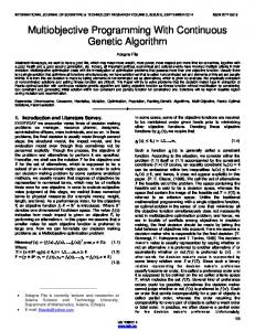
MPGA vs. MOGA in parallel machine scheduling problems with three objectives Now let’s raise the challenge to the highest level by comparing MPGA with MOGA in
scheduling problems with three objectives, Makespan, TWT, and Total Weighted Completion time (TWC). The center point of four factors described in table 2 is used as the test problem. Ten instances are generated using different seed numbers. Each algorithm is simulated 10 times for each instance to obtain the averages. The parameters for both algorithms remain the same except for population size. For MPGA, six additional populations are added to the program for the objective of TWC, and the total number of populations is 26 (6x3+8). The same number of populations is then used by MOGA. The results are shown in table 7. MPGA outperforms MOGA both quantitatively and qualitatively. MPGA’s qualitative performance increases slightly from 60.7% of two objective-scheduling problems to 66.9% of three-objective scheduling problems. Figure 5 illustrates the comparison of MPGA with MOGA in one simulation of one instance. Two dimensional figures are used to represent the Pareto Front solutions of both algorithms. For Makespan-TWC and Makespan-TWC comparisons, MPGA clearly produces better solutions than MOGA. The TWT-TWC solutions of both algorithms do not follow the concave-shape curves like others. This is mainly because of the highly correlation between TWC and TWT. In spite of this irregular shape, MPGA still outperforms MOGA in the TWC-TWT comparison. 15
5.
Conclusions and Future Work Solving a NP-hard scheduling problem with only one objective is a difficult task.
Heuristics have been developed to get near optimal solutions. Adding more objectives obviously makes this problem more difficult to solve. This paper presents a new methodology, the twostage Multiple Population Genetic Algorithm (MPGA) by improving and combining two heuristics, Vector Evaluation Genetic Algorithm (VEGA) and Multiple Objective Genetic Algorithm (MOGA). In the first stage, all of the objectives are combined into a single objective so that the algorithm can converge quickly and produce good solutions with respect to all the objectives. The solutions of the first stage are then divided into several sub-populations that evolve separately. The solutions for each objective can be improved for the individual sub-populations while another set of populations contains solutions satisfying the combined objective. Computational results show that the two-stage MPGA outperforms MOGA in most of the test problems with two objectives.
An extended study in the three-objective parallel machine
scheduling problem also indicates the superiority of the two-stage MPGA to the MOGA. Although the MPGA approach in this study is used to solve scheduling problems, it can be easily applied to other optimization problems by changing the encoding scheme of a GA. The two-stage MPGA shows good results compared to that of MOGA, but both algorithms seem to produce many unwanted solutions that are dominated by other solutions. This is caused by the high complexity of the problems studied in this paper. A more advanced genetic algorithm needs to be developed to take this issue into consideration. In addition, high variance among iterations of the genetic algorithm is observed; this is a problem for every GA researcher. Reducing the variance among the iterations of the genetic algorithm is another 16
research direction so that the solution of any iteration of the genetic algorithm will fall within a desirable range. In addition, to compare more than two algorithms by one single measure, a better performance measure needs to be developed. This measure should also be able to consider the case when objectives are not equally weighted. The results of this research will be reported shortly.
6.
Acknowledgements The authors gratefully acknowledge the support of the National Science Foundation
(Grant DMI-9713750) and the Semiconductor Research Corporation (Contract 97-EJ-492).
References [1]
Pinedo M. Scheduling: Theory, Algorithms, and Systems, Prentice Hall, New Jersey, 1995.
[2]
Gross D, Harris CM. Fundamentals of Queueing Theory, 3rd edition, John Wiley & Sons, New York, 1988.
[3]
Rosenthal RE.
Concepts, theory, and techniques - principle of multiobjective
optimization. Decision Science 1985; 16:133-152. [4]
Fry TD, Armstrong RD, Lewis H. A framework for single machine multiple objective sequencing research. Omega 1989; 17:594-607.
[5]
Lee C-Y, Vairaktarakis GL. Complexity of single machine hierarchical scheduling: a survey. in Complexity in Numerical Optimization, Pardalos PM., ed., World Scientific Publishing 1993; 269-298.
17
[6]
Lee SM, Jung H-J.
A multi-objective production planning model in a flexible
manufacturing environment.
International Journal of Production Research 1989;
27:1981-1992. [7]
Schaffer JD. Multiple objective optimization with vector evaluated genetic algorithms. Proceedings of the first ICGA 1985; 93-100.
[8]
Murata T, Ishibuchi H, Tanaka H. Multi-objective genetic algorithm and its application to flowshop scheduling. Computers and Industrial Engineering 1996; 30:957-968.
[9]
Hyun CJ, Kim Y, Kin YK. A genetic algorithm for multiple objective sequencing problems in mixed model assembly. Computers and Operations Research 1998; 25:675690.
[10]
Omori R, Sakakibara Y, Suzuki A. Applications of genetic algorithms to optimization problems in the solvent extraction process for spent nuclear fuel. Nuclear Technology 1997; 118:26-31.
[11]
Chen Y, Narita M., Tsuji M, Sa S. A genetic algorithm approach to optimization for the radiological worker allocation problem. Health Physics 1996; 70:180-186.
[12]
Marett R, Wright M.
A comparison of neighborhood search techniques for multi-
objective combinatorial problems. Computers and Operations Research 1996; 23:465483. [13]
Yim SJ, Lee DY. Multiple objective scheduling for flexible manufacturing systems using petri nets and heuristic search. Proceedings IEEE International Conference on Systems, Man, and Cybernetics 1996; 4:2984-2989.
[14]
Jaszkiewicz A.
A metaheuristic approach to multiple objective nurse scheduling.
Foundations of Computing and Decision Sciences 1997; 22:169-183. 18
[15]
Cieniawski SE, Eheart JW, Ranjithan S.
Using genetic algorithms to solve a
multiobjective groundwater monitoring problem. Water Resources Research 1995; 31:399-409. [16]
Fowler JW, Horng S-M, Cochran JK. A hybridized genetic algorithm to solve parallel machine problem scheduling problem with sequence dependent setups. International Journal of Manufacturing Technology and Management 2000; 1:3/4.
19
Encoding Initialization Selection Crossover Stage 1 Mutation Evaluation of combined objective Elitist Turing criteria No
Yes Re- initialization
Population 1 for objective 1
Population N for objective N
Population N+1 for combined objective
Selection
Selection
Selection
Crossover
Crossover
Crossover
Mutation
Mutation
Mutation
Stage 2
Elitist strategy Stopping criteria Yes
No Stop
Figure 1. A two-stage Multi-Population Genetic Algorithm (MPGA) for multi-objective scheduling problems.
20
900 1 4
Makespan
880
2 5
3 6
860 840 820 800 0
1000
2000
3000
4000
5000
Generation
Figure 2. Comparison Pareto Front average of makespan of six functions.
48000 1 4
TWT
44000
2 5
3 6
40000 36000 32000 28000 0
1000
2000
3000
4000
5000
Generation Figure 3. Comparison Pareto Front average of TWT of six functions.
21
1 Makespan TWT
0.8 0.6 0.4 0.2 0 0
1000
2000
3000
4000
5000
Generation
Figure 4. Performance of different turn points as optimizing makespan and TWT.
22
MPGA MOGA
130000 110000 90000 70000 720
Makespan
TWC
150000
820 800 780 760 740 720 230000
740
760 780 Makespan
800
820
MPGA MOGA
250000
270000
290000
TWT
MPGA 290000
MOGA
270000 250000 230000 70000
90000 110000 130000 150000 TWC
Figure 5. Comparison of MPGA with MOGA
23
Table 1. Six objective functions of multiple objective in scheduling problem Case Objective Function n
f t , j ( x ) = ∑ f t ,i , j ( x )
1
i =1 n
f t , j ( x ) = ∑ wt ,i f t , i , j ( x )
2
i =1
3
n f (x ) f t , j ( x ) = ∑ t ,i , j * f t , i , j ( x ) i =1
4
n f (x ) f t , j ( x ) = ∑ wt ,i t ,i , j * f t , i , j ( x ) i =1
5
n f (x ) f t , j ( x ) = ∏ t ,i , j * f t , i , j ( x ) i =1
6
f t ,i , j ( x ) − f * t , i , j ( x ) f t , j ( x ) = ∑ * ( ) f t ,i , j x i =1 n
(
)
where f *t, i ( x ) is the best solution of objective i at generation t. Table 2. Characteristics of test problem •
Factors Range of weights
•
Range of due dates
•
Ratio ( p
•
WIP status
s
)
Levels Narrow Wide Narrow Wide High Moderate Low High Moderate Low
Description [1,10]. [1,20]. Release time + [-1,2] x total process time. Release time + [-2,4] x total process time. 50/10, p = 50+[-9,9], s = 2*[3,7]. 30/30, p = 30+[-9,9], s = 6*[3,7]. 10/50, p = 10+[-9,9], s = 10*[3,7]. All jobs are ready at time 0. 50% of jobs are ready at time 0 and the others are ready at time [0,720]. All jobs are ready at time [0,720].
Table 3. Example to calculate the quantitative and qualitative measures of two algorithms. Algorithms A B Number of solutions of Pareto Front 5 8 Number of solutions of combined Pareto Front 6 6 Number of solutions form the combined Pareto Front 2 4 Quantitative measure 5 8 Qualitative measure 2/6 4/6 24
Table 4. Comparison of MPGA and MOGA at quantitative and qualitative measures Quantitative Qualitative MPGA MOGA Prob # Weight Due Ratio WIP MPGA MOGA Win MPGA MOGA (%) (%) Win 1 N N H H 11.88 9.39 9.5 6.62 5.16 56.2 43.8 5.5 2 N N H M 11.98 9.52 9.5 8.18 4.15 66.3 33.7 8.5 3 N N H L 10.69 8.37 8.5 7.90 2.46 76.3 23.7 10 4 N N M H 11.74 8.79 10 6.02 5.38 52.8 47.2 6 5 N N M M 5.70 4.55 8 3.51 1.87 65.2 34.8 8 6 N N M L 6.95 5.40 9 4.41 2.32 65.5 34.5 9 7 N N L H 12.56 8.64 9 5.75 5.55 50.9 49.1 3 8 N N L M 1.82 1.22 9.5 0.61 0.72 45.9 54.1 3 9 N N L L 2.93 1.85 8 1.17 1.06 52.5 47.5 6 10 N W H H 11.99 9.70 8.5 7.31 4.74 60.7 39.3 7.5 11 N W H M 14.05 9.45 10 9.53 4.04 70.2 29.8 9 12 N W H L 10.8 8.92 9 7.91 2.95 72.8 27.2 10 13 N W M H 11.4 9.15 9.5 5.99 5.38 52.7 47.3 6 14 N W M M 6.67 4.76 8 3.92 2.01 66.1 33.9 8 15 N W M L 7.88 5.29 10 5.02 2.46 67.1 32.9 8 16 N W L H 12.5 9.53 10 5.67 6.13 48.1 51.9 4 17 N W L M 2.06 1.27 9 0.81 0.70 53.6 46.4 6 18 N W L L 4.33 1.94 9.5 1.48 1.28 53.6 46.4 5 19 W N H H 12.15 8.86 10 6.61 4.78 58.0 42.0 5 20 W N H M 13.32 9.38 9.5 9.69 3.70 72.4 27.6 9.5 21 W N H L 11.49 8.79 10 7.14 3.67 66.0 34.0 8.5 22 W N M H 11.91 8.71 10 6.73 4.53 59.8 40.2 6 23 W N M M 5.74 4.77 5.5 3.68 1.38 72.7 27.3 9 24 W N M L 8.17 5.35 10 4.52 2.69 62.7 37.3 7 25 W N L H 12.57 9.30 9.5 5.97 6.00 49.9 50.1 4.5 26 W N L M 1.59 1.27 8 0.69 0.66 51.1 48.9 5 27 W N L L 3.30 1.99 9 1.31 1.13 53.7 46.3 6 28 W W H H 12.44 9.31 8.5 6.91 4.90 58.5 41.5 7 29 W W H M 13.81 9.42 9.5 10.67 3.23 76.8 23.2 10 30 W W H L 11.85 9.24 9 8.87 3.04 74.5 25.5 10 31 W W M H 11.69 8.57 9 6.53 4.66 58.4 41.6 6 32 W W M M 7.46 5.15 6 5.00 1.77 73.9 26.1 9.5 33 W W M L 8.46 5.55 10 4.66 2.86 62.0 38.0 7 34 W W L H 12.88 9.58 9.5 6.09 6.00 50.4 49.6 5 35 W W L M 1.87 1.29 8.5 0.67 0.83 44.7 55.3 4.5 36 W W L L 4.18 2.00 10 1.75 1.04 62.7 37.3 5.5 Avg. 8.97 6.56 9.1 5.26 3.20 60.7 39.3 6.9 Note: the column of “Win” represents how many instances (out of 10) MPGA performs better than MOGA.
25
Table 5. Comparison of MPGA and MOGA based on the individual factor of test problems Quantitative Qualitative MPGA MOGA Weight Due Ratio WIP MPGA MOGA Win MPGA MOGA (%) (%) Win N 8.77 6.54 164.5 5.10 3.24 59.8 40.2 122.5 W 9.16 6.59 161.5 5.42 3.16 61.6 38.4 125 N 8.69 6.45 162.5 5.03 3.18 59.9 40.1 119.5 W 9.24 6.67 163.5 5.49 3.22 61.5 38.5 128 H 12.20 9.20 111.5 8.11 3.90 67.4 32.6 100.5 M 8.65 6.34 105 5.00 3.11 63.2 36.8 89.5 L 6.05 4.16 109.5 2.66 2.59 51.4 48.6 57.5 H 12.14 9.13 113 6.35 5.27 54.7 45.3 65.5 M 7.17 5.17 101 4.75 2.09 63.2 36.8 90 L 7.59 5.39 112 4.68 2.25 64.1 35.9 92 Note: the column of “Win” represents how many instances (out of 180 for factors Weight and Due, and out of 120 for factors Ratio and WIP) MPGA performs better than MOGA.
Table 6. Comparison of MPGA and MOGA based on two significant factors (ratio of average process times to average setup times and WIP status) of test problems Quantitative Qualitative MPGA MOGA Ratio WIP MPGA MOGA Win MPGA MOGA (%) (%) Win H H 12.12 9.32 36.5 6.86 4.90 58.4 41.6 25 H M 13.29 9.44 38.5 9.52 3.78 71.4 28.6 37 H L 11.21 8.83 36.5 7.96 3.03 72.4 27.6 38.5 M H 11.69 8.81 38.5 6.32 4.99 55.9 44.1 24 M M 6.39 4.81 27.5 4.03 1.76 69.5 30.5 34.5 M L 7.87 5.40 39 4.65 2.58 64.3 35.7 31 L H 12.63 9.26 38 5.87 5.92 49.8 50.2 16.5 L M 1.84 1.26 35.0 0.70 0.73 48.8 51.2 18.5 L L 3.69 1.95 36.5 1.43 1.13 55.6 44.4 22.5 Total 326 247.5 Note: the column of “Win” represents how many instances (out of 40) MPGA performs better than MOGA.
Table 7. Comparison of MPGA and MOGA for the scheduling problems with three objectives, Makespan, TWC, and TWT Quantitative Qualitative MPGA MOGA MPGA MOGA MPGA(%) MOGA(%) 13.94 10.65 8.78 4.34 66.9 33.1
26