Brandt, “Multi-level Adaptive Solutions to Boundary Value. Problems,” Math
Comp., 31, 1977, pp 333-390. • Brandt, “1984 Guide to Multigrid Development,
with.
A Multigrid Tutorial By William L. Briggs Presented by Van Emden Henson Center for Applied Scientific Computing Lawrence Livermore National Laboratory This work was performed, in part, under the auspices of the United States Department of Energy by University of California Lawrence Livermore National Laboratory under contract number W-7405-Eng-48.
Outline • Model Problems • Basic Iterative Schemes – Convergence; experiments – Convergence; analysis
• Development of Multigrid – – – –
Coarse-grid correction Nested Iteration Restriction and Interpolation Standard cycles: MV, FMG
• Performance – Implementation – storage and computation costs
• Performance, (cont) – Convergence – Higher dimensions – Experiments
• Some Theory – The spectral picture – The subspace picture – The whole picture!
• Complications – Anisotropic operators and grids – Discontinuous or anisotropic coefficients – Nonlinear Problems: FAS
2 of 119
Suggested Reading • Brandt, “Multi-level Adaptive Solutions to Boundary Value Problems,” Math Comp., 31, 1977, pp 333-390. • Brandt, “1984 Guide to Multigrid Development, with applications to computational fluid dynamics.” • Briggs, “A Multigrid Tutorial,” SIAM publications, 1987. • Briggs, Henson, and McCormick, “A Multigrid Tutorial, 2nd Edition,” SIAM publications, 2000. • Hackbusch, Multi-Grid Methods and Applications,” 1985. • Hackbusch and Trottenburg, “Multigrid Methods, SpringerVerlag, 1982” • Stüben and Trottenburg, “Multigrid Methods,” 1987. • Wesseling, “An Introduction to Multigrid Methods,” Wylie, 1992 3 of 119
Multilevel methods have been developed for... • Elliptic PDEs • Purely algebraic problems, with no physical grid; for example, network and geodetic survey problems. • Image reconstruction and tomography • Optimization (e.g., the travelling salesman and long transportation problems) • Statistical mechanics, Ising spin models. • Quantum chromodynamics. • Quadrature and generalized FFTs. • Integral equations. 4 of 119
Model Problems • One-dimensional boundary value problem:
0 < x < 1,
− u″ ( x ) + σ u( x ) = f ( x )
σ>0
u( 0) = u( 1 ) = 0 1 • Grid: h = N
, xi = ih ,
x =0
x0 x1 x2
• Let
v i ≈ u( x i )
xi
i = 0, 1 , . . . N x =1 xN
and f i ≈ f ( x i ) for i = 0, 1, . . . N 5 of 119
We use Taylor Series to derive an approximation to u’’(x) • We approximate the second derivative using Taylor series: 2 3
h h u( x i + 1 ) = u( x i ) + h u′ ( x i ) + u″ ( x i ) + u′′′ ( x i ) + O( h 4 ) 2! 3!
h2 h3 u( x i − 1 ) = u( x i ) − h u′ ( x i ) + u″ ( x i ) − u′′′ ( x i ) + O( h 4 ) 2! 3!
• Summing and solving,
u″ ( x i ) =
u( x i + 1 ) − 2 u( x i ) + u( x i − 1 ) h2
+ O( h 2)
6 of 119
We approximate the equation with a finite difference scheme • We approximate the BVP
− u″ ( x ) + σ u( x ) = f ( x )
0 < x < 1,
σ>0
u( 0) = u( 1 ) = 0 with the finite difference scheme:
− vi − 1 + 2 vi − vi + 1 h2
+ σ vi = f i
i = 1, 2, . . . N − 1
v0 = vN = 0 7 of 119
The discrete model problem T v = ( v , v , . . . , v ) • Letting 1 2 N − 1 and
f
= ( f 1, f 2, . . . , f N − 1 ) T
we obtain the matrix equation A v = f where A is (N-1) x (N-1), symmetric, positive definite, and ö æ 2 + σh2 −1 ÷ ç 2 ÷ ç − 1 2 + σh −1 ÷ ç 2 1 ç ÷ − 1 2 + σh − 1 A= ÷, 2 ç h ç ÷ ÷ ç 2 h − + σ − 1 2 1 ÷ ç ç 2÷ − 1 2 + σh ø è
æ v1 ö ç v2 ÷ ç ÷ ç v3 ÷ v= ç ÷, ÷ ç v ç N −2 ÷ ÷ çv 1 N − è ø
æ f1 ö ç f ÷ ç 2 ÷ ç f ÷ f =ç 3 ÷ ç ÷ ç f N −2÷ ç ÷ f è N −1ø 8 of 119
Solution Methods • Direct – Gaussian elimination – Factorization
• Iterative – Jacobi – Gauss-Seidel – Conjugate Gradient, etc.
• Note: This simple model problem can be solved very efficiently in several ways. Pretend it can’t, and that it is very hard, because it shares many characteristics with some very hard problems. 9 of 119
A two-dimensional boundary value problem • Consider the problem:
0 < x < 1, 0 < y < 1 − ux x − uyy + σ u = f ( x , y ) , u = 0 , x = 0, x = 1, y = 0, y = 1; σ>0 • Where the grid is given: hx =
z
1 1 , hy = , M N
( x i , yj ) = ( i hx , j hy )
0≤ i ≤ M
y
0≤ j ≤ N
x
10 of 119
Discretizing the 2D problem • Let v i j ≈ u( x i , yj ) and f i j ≈ f ( x i , yj ) . Again, using 2nd order finite differences to approximate u x x and uy y we obtain the approximate equation for the unknown u( x i , yj ) , for i=1,2, … M-1 and j=1,2, …, N-1: − v i − 1, j + 2v i j − v i + 1, j hx2
+
− v i , j − 1 + 2v i j − v i , j + 1 hy2
+ σ vi j = f i j
v i j = 0 , i = 0, i = M , j = 0, j = M
• Ordering the unknowns (and also the vector f ) lexicographically by y-lines: v = ( v 1, 1 , v 1, 2 , . . . , v 1, N − 1 , v 2, 1 , v 2, 2 , . . . v 2, N − 1, . . . , v N − 1, 1, v N − 1, 2 , . . . , v N − 1, N − 1 ) T
11 of 119
Yields the linear system • We obtain a block-tridiagonal system Av = f : æ A1 − Iy ö ç −I A ÷ − I y y 2 ç ÷ ç ÷ − Iy A3 − Iy ç ÷ ç ÷ − Iy AN − 2 − Iy ÷ ç ç ÷ − I A y N −1 ø è
æ f1 ö v1 ö æ ç ÷ f v ç 2 ÷ ç 2 ÷ ç v3 ÷ ç f ÷ 3 = ÷ ç ç ÷ ç ÷ ÷ ç ç ÷ ÷ ç çf ÷ è vN − 1 ø è N −1 ø 1
where Iy is a diagonal matrix with diagonal and 1 1 æ 1 + +σ − ç 2 2 ç h x hy ç 1 ç − ç hx2 ç ç Ai = ç ç ç ç ç ç ç ç è
on the
hy2
hx2
1 h x2
+ −
1 h y2
+σ
−
1
1
hx2
hx2
+
1 h x2 1
h y2 ⋅⋅ ⋅
+σ
−
1 h x2
⋅⋅ −
⋅ 1
1
hx2 h x2
ö ÷ ÷ ÷ ÷ ÷ ÷ ÷ ÷ ÷ ÷ ÷ ⋅⋅ ÷ ⋅ ÷ 1 + +σ÷ ÷ hy2 ø
12 of 119
Iterative Methods for Linear Systems • Consider Au = f where A is NxN and let v be an approximation to u. • Two important measures: – The Error:
e = u−v ,
|| e ||∞ = max | ei | – The Residual:
with norms
|| e ||2 =
å
N 2 e i =1 i
r = f − A v with || r ||2 || r ||∞ 13 of 119
Residual correction • Since e = u − v , and r = f − A v , we can write A u = f as
A ( v + e) = f
which means that A e Residual Equation:
= f − Av
, which is the
Ae = r
• Residual Correction:
u = v +e 14 of 119
Relaxation Schemes • Consider the 1D model problem − ui − 1 +2 ui − ui + 1 = h 2 f i
1 ≤ i ≤ N −1
u0 = uN = 0
• Jacobi Method (simultaneous displacement): Solve the ith equation for v i holding other variables fixed: 1 ( o ld) ( n e w ) vi = ( v i − 1 + v i( +ol1d) + h 2 f i ) 1 ≤ i ≤ N −1 2
15 of 119
In matrix form, the relaxation is • Let A = ( D − L − U ) where D is diagonal and L and U are the strictly lower and upper parts of A. • Then
Au = f
becomes
(D −L −U) u = f D u = ( L + U) u + f
u =D
−1
( L + U) u + D
−1
f
−1 • Let R J = D ( L + U), then the iteration is: v ( n ew) = R J v ( o ld ) + D − 1 f 16 of 119
The iteration matrix and the error
• From the derivation, u = D − 1 ( L + U) u + D − 1 f u = RJ u + D − 1 f • the iteration is
v ( n ew) = R J v ( o ld ) + D − 1 f • subtracting, • or
u − v ( n ew) = R J u + D − 1 f − ( R J v ( o ld) + D − 1 f )
• hence
u − v ( n ew) = R J u − R J v ( o ld) e ( n ew) = R J e ( o ld) 17 of 119
Weighted Jacobi Relaxation • Consider the iteration:
ω ( o ld ) ( n e w ) ( o l d ) vi ← ( 1 − ω) v i + ( v i − 1 + v i( +o l1d) + h 2f i ) 2
• Letting A = D-L-U, the matrix form is: v ( n ew) = ( 1 − ω) I + ω D − 1( L + U) v ( o ld) + ω h 2D − 1f
= R ω v ( o ld) + ω h 2D − 1f • Note that
.
R ω = [ ( 1 − ω) I +ω R J ]
• It is easy to see that if e ≡ u ( ex a c t ) − u then e ( n ew) = R ω e ( o ld)
( a pp ro x )
,
18 of 119
Gauss-Seidel Relaxation (1D) • Solve equation i for ui and update immediately. • Equivalently: set each component of r to zero. • Component form: for i = 1, 2, . . . N − 1, set 1 vi ← ( vi − 1 + vi + 1 + h 2 f i ) 2
• Matrix form:
A = (D −L −U)
( D − L) u = U u + f u = ( D − L) − 1 U u + ( D − L) − 1 f
• Let R G = ( D − L ) − 1U • Then iterate v ( n ew) ← R G v ( old) + ( D − L ) − 1f • Error propagation: e ( n ew) ← R G e ( o ld)
19 of 119
Red-Black Gauss-Seidel • Update the even (red) points 1 v 2i ← ( v 2i − 1 + v 2i + 1 + h 2 f 2i ) 2
• Update the odd (black) points v 2i + 1 ←
x0
1 ( v 2i + v 2i + 2 + h 2 f 2i + 1 ) 2
xN
20 of 119
Numerical Experiments • Solve A u = 0 , − ui − 1 + 2 ui − ui + 1 = 0 • Use Fourier modes as initial iterate, with N =64: vk
æ ikπ ö = ( v i ) k = sin ç ÷ N ø è
1 ≤ i ≤ N − 1,
component
1 ≤ k ≤ N −1
mode
k =1 1
k =3
0 .8 0 .6 0 .4 0 .2 0
k =6
-0 . 2 -0 . 4 -0 . 6 -0 . 8 -1 0
0 .1
0 .2
0 .3
0 .4
0 .5
0 .6
0 .7
0 .8
0 .9
1
21 of 119
Error reduction stalls • Weighted ω = 32 Jacobi on 1D problem. • Initial guess: v = 1 æ sin æ j π ö + sin æ 6 j π ö + sin æ 32 j π ö 0
3 çè
ç N ÷ ø è
ö ç N ÷ ÷ ø ø è
ç N ÷ ø è
• Error || e ||∞ plotted against iteration number: 1 0 .9 0 .8 0 .7 0 .6 0 .5 0 .4 0 .3 0 .2 0 .1 0 0
10
20
30
40
50
60
70
80
90
100
22 of 119
Convergence rates differ for different error components • Error, ||e||∞ , in weighted Jacobi on Au = 0 for 100 iterations using initial guesses of v1, v3, and v6 k =1
1 0.9 0.8 0.7 0.6 0.5
k =3
0.4 0.3
k =6
0.2 0.1 0 0
20
40
60
80
100
120
23 of 119
Analysis of stationary iterations • Let v ( new) = R v ( old) + g . The exact solution is unchanged by the iteration, i.e., u = R u + g. • Subtracting, we see that
e ( n ew) = R e ( o ld) • Letting e0 be the initial error and ei be the error after the ith iteration, we see that after n iterations we have
e ( n ) = R n e ( 0) 24 of 119
A quick review of eigenvectors and eigenvalues • The number λ is an eigenvalue of a matrix B, and w its associated eigenvector, if Bw = λ w. • The eigenvalues and eigenvectors are characteristics of a given matrix. • Eigenvectors are linearly independent, and if there is a complete set of N distinct eigenvectors for an NxN matrix, they form a basis; i.e., for any v, there exist unique ck such that: v =
N
å ck wk
k =1
25 of 119
“Fundamental theorem of iteration” • R is convergent (that is, R n → 0 as n → ∞) if and only if ρ ( R ) < 1 , where ρ ( R ) = ma x { | λ1 | , | λ2 | , ... , | λN | }
therefore, for any initial vector v(0), we see that e ( n ) → 0 a s n → ∞ if and only if ρ ( R ) < 1. • ρ ( R ) < 1 assures the convergence of the iteration given by R and ρ ( R ) is called the convergence factor for the iteration. 26 of 119
Convergence Rate • How many iterations are needed to reduce the initial error by 10 − d ? || e ( M ) || || e ( 0) ||
≤ || R M || ∼ ( ρ ( R ) ) M ∼ 10 − d
• So, we have M =
d æ 1 ö l og10 ç ρ( R) ÷ è ø
.
• The convergence rate is given:
æ 1 ö ra t e = l og10 ç ÷ ρ ( ) R è ø
= − l og10 ( ρ ( R ) )
digit s it er a t ion 27 of 119
Convergence analysis for weighted Jacobi on 1D model R ω = ( 1 − ω) I + ω D − 1( L + U ) = I − ωD − 1 A
æ 2 −1 ö ÷ ç −1 2 −1 ÷ ωç 1 2 1 − − Rω = I − ç ÷ 2ç ⋅⋅ ⋅⋅ ⋅⋅ ÷ ⋅÷ ⋅ ⋅ ç −1 2 ø è
ω λ ( Rω ) = 1 − λ ( A) 2
For the 1D model problem, he eigenvectors of the weighted Jacobi iteration and the eigenvectors of the matrix A are the same! The eigenvalues are related as well. 28 of 119
Good exercise: Find the eigenvalues & eigenvectors of A • Show that the eigenvectors of A are Fourier modes! j kπ ö k π æ æ ö wk , j = sin ç λk ( A ) = 4 sin2 ç , ÷ ÷ 2 N N è ø è ø 1
1
1
0 .8
0 .8
0 .8
0 .6
0 .6
0 .6
0 .4
0 .4
0 .4
0 .2
0 .2
0 .2
0
0
0
-0 . 2
-0 . 2
-0 . 2
-0 . 4
-0 . 4
-0 . 4
-0 . 6
-0 . 6
-0 . 6
-0 . 8
-0 . 8
-0 . 8
-1
-1 0
10
20
30
40
50
60
-1 0
10
20
30
40
50
60
0
10
20
30
40
50
60
1 1
0 .8
0 .8
0 .6
0 .6
0 .4 0 .4
0 .2 0 .2
0
0
-0 . 2
-0 . 2 -0 . 4
-0 . 4
-0 . 6
-0 . 6
-0 . 8
-0 . 8
-1
-1 0
10
20
30
40
50
60
0
10
20
30
40
50
60
29 of 119
Eigenvectors of Rω and A are the same,the eigenvalues related kπ ö λk ( R ω ) = 1 − ç 2N ÷ ø è • Expand the initial error in terms of the N −1 eigenvectors: æ 2 2 ω sin
e ( 0) =
å
k =1
c k wk
• After M iterations, R M e ( 0)
=
N −1
å
k =1
ck R
M
wk =
N −1
å
k =1
c k λM k wk
• The kth mode of the error is reduced by λk at each iteration
30 of 119
Relaxation suppresses eigenmodes unevenly • Look carefully at 1
æ kπ ö λk ( R ω ) = 1 − 2 ω sin2 ç ÷ 2 N è ø
0.8
ω = 1/3
0.6
k = 1, 2, . . . , N − 1
Eigenvalue
0.4
ω = 1/ 2
0.2 0
For 0 ≤ ω ≤ 1,
N 2
-0.2 -0.4
Note that if 0 ≤ ω ≤ 1 then | λk ( R ω ) | < 1 for
ω=1
ω = 2/ 3
-0.6 -0.8 -1 k
æ π ö λ1 = 1 − 2 ω sin2 ç ÷ 2 N è ø
æ πh ö = 1 − 2 ω s in 2 ç ÷ 2 è ø
= 1 − O ( h2) ≈ 1 31 of 119
Low frequencies are undamped • Notice that no value of ω will damp out the long (i.e., low frequency) waves. 1 0.8
ω = 1/3
0.6
Eigenvalue
0.4
N ≤ k ≤ N 2
ω = 1/ 2
0.2 0
N 2
-0.2 -0.4
What value of ω gives the best damping of the short waves ?
ω=1
ω = 2/ 3
-0.6 -0.8
Choose ω such that
λN ( R ω ) = − λN ( R ω ) 2
-1 k
2 Þ ω= 3 32 of 119
The Smoothing factor • The smoothing factor is the largest absolute value among the eigenvalues in the upper half of the spectrum of the iteration matrix N f or ≤ k≤ N 2
smoot hing f a ct or = ma x λk ( R )
• For Rω, with ω = since
λN 2
• But,
= λN
1 2 , the smoothing factor is 3 , 3 1 = 3
and
2 λk ≈ 1 − k 2 π2 h 2 3
λk
N/2, the kth mode on the fine grid is aliased and appears as the (N-k)th mode on the coarse grid: æ ( 2j ) πk ö h ( wk ) = s in ç ÷ 2j N è ø
æ 2πj ( N − k ) ö = − sin ç ÷ N ø è
1 0 .8 0 .6 0 .4 0 .2 0 -0 . 2 -0 . 4 -0 . 6 -0 . 8 -1 0
2
4
6
8
10
12
5
6
k=9 mode, N=12 grid 1 0 .8 0 .6 0 .4 0 .2
æ π ( N − k) j ö = − s in ç ÷ N / 2 è ø
= −(
wN2h− k )
0 -0 . 2 -0 . 4 -0 . 6 -0 . 8 -1 0
1
2
3
4
k=3 mode, N=12 grid
43 of 119
Second observation toward multigrid: • Recall the residual correction idea: Let v be an approximation to the solution of Au=f, where the residual r=f-Av. The the error e=u-v satisfies Ae=r. • After relaxing on Au=f on the fine grid, the error will be smooth. On the coarse grid, however, this error appears more oscillatory, and relaxation will be more effective. • Therefore we go to a coarse grid and relax on the residual equation Ae=r, with an initial guess of e=0. 44 of 119
Idea! Coarse-grid correction • Relax on Au=f on
Ω h to obtain an approximation v h
• Compute r = f − A v h . 2h • Relax on Ae=r on Ω to obtain an approximation to the error, e 2h . • Correct the approximation v h ← v h + e 2h . • Clearly, we need methods for the mappings h 2h and Ω 2h Ωh
Ω
Ω
45 of 119
1D Interpolation (Prolongation) • Mapping from the coarse grid to the fine grid: I 2hh : Ω 2h → Ω h • Let v h , v 2h
be defined on Ω h, Ω 2h. Then
I 2hh v 2h = v h where
v 2hi = v i2h 1 2h h v 2i + 1 = ( v i + v i2h+ 1 ) 2
for
N 0≤i ≤ −1 2 46 of 119
1D Interpolation (Prolongation) • Values at points on the coarse grid map unchanged to the fine grid • Values at fine-grid points NOT on the coarse grid are the averages of their coarse-grid neighbors
Ω 2h
Ω
h
47 of 119
The prolongation operator (1D) h I • We may regard 2h as a linear operator from
ℜN/2-1
• e.g., for N=8,
•
ℜN-1
ö æ 1/2 ÷ ç 1 ÷ ç 2h ÷ æ v1 ç 1/2 1/2 ÷ ç 2h ç 1 ÷ ç v2 ç ÷ ç 2h ç / / 1 2 1 2 ÷ è v3 ç ç 1 ÷ ÷ ç / 1 2 ø 7x 3 è
æ v 1h ç ç v 2h ç ö ç v 3h ÷ ç h = ç v4 ÷ ç h ÷ ç v5 ø 3x 1 ç h ç v6 ç vh è 7
ö ÷ ÷ ÷ ÷ ÷ ÷ ÷ ÷ ÷ ÷ ÷ ø 7x 1
I 2hh has full rank, and thus null space { φ }
48 of 119
How well does v2h approximate u? • Imagine that a coarse-grid approximation v2h has been found. How well does it approximate the exact solution u ? Think u error!!
• If u is smooth, a coarse-grid interpolant of v2h may do very well. 49 of 119
How well does v2h approximate u? • Imagine that a coarse-grid approximation v2h has been found. How well does it approximate the exact solution u ? Think u error!!
• If u is oscillatory, a coarse-grid interpolant of v2h may not work well. 50 of 119
Moral of this story: • If u is smooth, a coarse-grid interpolant of v2h may do very well. • If u is oscillatory, a coarse-grid interpolant of v2h may not work well. • Therefore, nested iteration is most effective when the error is smooth!
51 of 119
1D Restriction by injection
• Mapping from the fine grid to the coarse grid: I h2h : Ω h → Ω 2h
• Let v h , v 2h be defined on Ω h, Ω 2h . Then where v i2h = v 2hi .
I h2h v h = v 2h
52 of 119
1D Restriction by full-weighting h 2h • Let v h , v 2h be defined on Ω , Ω . Then
where
I h2h v h = v 2h 1 h 2 h v i = ( v 2i − 1 + 2 v 2hi + v 2hi + 1 ) 4
53 of 119
The restriction operator R (1D) 2h • We may regard I h as a linear operator from
ℜN-1
• e.g.,
ℜN/2-1
æ v 1h ç for N=8, ç v 2h ç ç v 3h 1/4 1/2 1/4 æ öç h 1/4 1/2 1/4 ç ÷ ç v4 è 1/4 1/2 1/4 ø ç v h ç 5 ç h ç v6 ç vh è 7
ö ÷ ÷ ÷ æ v 12h ö ÷ ç 2h ÷ ÷ = ç v2 ÷ ÷ ÷ ç 2h ÷ ÷ è v3 ø ÷ ÷ ÷ ø
N 2h N • I h has rank ∼ , and thus dim(NS(R)) ∼ 2 2
54 of 119
Prolongation and restriction are often nicely related • For the 1D examples, linear interpolation and fullweighting are related by: æ1 ö ç2 ÷ ç ÷ ç1 1 ÷ 1 ç ÷ I 2hh = ç 2 ÷ 2 ç ÷ 1 1 ç ÷ ç 2÷ ç ÷ 1ø è
1æ 2h Ih = ç 4 è
1 2 1 ö 1 2 1 ÷ 1 2 1 ø
• A commonly used, and highly useful, requirement is that h 2h T I 2h = c ( I h )
for c in
ℜ 55 of 119
2D Prolongation v 2hi, 2j = v i2jh 1 2h h v 2i + 1, 2j = ( v i j + v ih+ 1, j ) 2 v 2hi , 2j + 1 = v 2hi + 1, 2j + 1
1 2h ( v i j + v ih, j + 1 ) 2 1 = ( v i2jh + v ih+ 1, j + v ih, j + 1 + v ih+ 1, j + 1 ) 4
1 4 1 2 1 4
1 2 1 1 2
1 4 1 2 1 4
We denote the operator by using a “give to” stencil, ] [. Centered over a c-point, , it shows what fraction of the c-point’s value is contributed to neighboring f-points, . 56 of 119
2D Restriction (full-weighting) 1 16 1 8 1 16
1 8 1 4 1 8
1 16 1 8 1 16
We denote the operator by using a “give to” stencil, [ ]. Centered over a c-point, , it shows what fractions of the neighboring ( ) f-points’ value is contributed to the value at the c-point. 57 of 119
Now, let’s put all these ideas together • Nested Iteration (effective on smooth error modes) • Relaxation (effective on oscillatory error modes) • Residual equation (i.e., residual correction) • Prolongation and Restriction
58 of 119
Coarse Grid Correction Scheme v h ← CG ( v h, f h , α1 , α2 )
• 1) Relax α1 times on A h u h = f h on Ω h with arbitrary initial guess v h . h h • 2) Compute r h = f − A v h.
2h • 3) Compute r 2h = I h r.h
2h • 4) Solve A e 2h = r 2h on Ω 2h . h ← v h + I h e 2h v • 5) Correct fine-grid solution . 2h
• 6) Relax α2 times on A h u h = f h on Ω h with initial guess v h . 59 of 119
Coarse-grid Correction h h h A u = f Relax on h = f h −Ahuh r Compute
uh ←
Correct u h + eh
Interpolate
Restrict r 2h = I h2h r h
eh
h 2h ≈ I2h e
2h Solve A e2h = r2h e 2h = ( A 2h) − 1 r 2h
60 of 119
What is
A
2h
?
2h
• For this scheme to work, we must have A , a coarse-grid operator. For the moment, we will 2h simply assume that A is “the coarse-grid h version” of the fine-grid operator A . 2h A • We will return to the question of constructing
later.
61 of 119
How do we “solve” the coarsegrid residual equation? Recursion! uh ← Gν ( Ah, f h )
uh ←uh + eh
eh ←I2hh u2h
f 2h ← Ih2h ( f h − Ahuh )
u2h ← Gν ( A2h, f 2h )
u2h ←u2h + e2h
f 4h ←I24hh( f 2h − A2hu2h )
e2h ←I42hh u4h u4h ←u4h + e4h
u4h ← Gν ( A4h, f 4h )
f 8h ←I48hh( f 4h − A4hu4h ) u8h ← Gν ( A8h, f 8h )
e4h ←I84hh u8h u8h ←u8h + e8h
eH = ( AH) −1f H
62 of 119
V-cycle (recursive form) v h ← MV h ( v h , f h )
h h h A u = f α 1) Relax 1 times on , initial v h arbitrary
2) If
Ω his the coarsest grid, go to 4)
Else:
f 2h ← I 2hh ( f h − A h v h ) v 2h ← 0
v 2h ← M V 2h ( v 2h , f 2h )
3) Correct
v h ← v h + I 2hh v 2h
h h 4) Relax α2 times on A u
h
= f , initial guess v h 63 of 119
h h Storage Costs: v and f must
be stored on each level
●
In 1-d, each coarse grid has about half the number of points as the finer grid.
● In 2-d, each coarse grid has about one-
fourth the number of points as the finer grid.
● In d-dimensions, each coarse grid has
about 2 − d the number of points as the finer grid. d
● Total storage cost: 2N ( 1 + 2
−d
+2
− 2d
+2
− 3d
+ …+2
− Md
)