Jun 30, 2014 - MARK F. ADAMS, JED BROWN, MATT KNEPLEY, AND RAVI SAMTANEY. Abstract. We investigate a technique â segmental refinement (SR) ...
SEGMENTAL REFINEMENT: A MULTIGRID TECHNIQUE FOR DATA LOCALITY
arXiv:1406.7808v1 [math.NA] 30 Jun 2014
MARK F. ADAMS, JED BROWN, MATT KNEPLEY, AND RAVI SAMTANEY Abstract. We investigate a technique – segmental refinement (SR) – proposed by Brandt in the 1970s as a low memory multigrid method. The technique is attractive for modern computer architectures because it provides high data locality, minimizes network communication, is amenable to loop fusion, and is naturally highly parallel and asynchronous. The network communication minimization property was recognized by Brandt and Diskin in 1994; we continue this work by developing a segmental refinement method for a finite volume discretization of the 3D Laplacian on massively parallel computers. An understanding of the asymptotic complexities, required to maintain textbook multigrid efficiency, are explored experimentally with a simple SR method. A two-level memory model is developed to compare the asymptotic communication complexity of a proposed SR method with traditional parallel multigrid. Performance and scalability are evaluated with a Cray XC30 with up to 64K cores. We achieve modest improvement in scalability from traditional parallel multigrid with a simple SR implementation.
1. Introduction Full multigrid (FMG) is a provably asymptotically exact, non-iterative, algebraic equation solver with work complexity of about five residual calculation for the constant coefficient Laplacian – textbook multigrid efficiency. Multigrid has been developed for many applications in the past 40 years and continues to be an active area of research and development. Textbook multigrid efficiency, or nearly so, has been observed experimentally in many applications [BD81, TDB01, TOS01, ASB10]. FMG is a highly parallel algorithm with a computational depth of log2 n, where n is the number of equations; the theoretical lower bound for solving that Laplacian is log n. While textbook multigrid efficiency is only provable for a few classes of problems, FMG is applied widely in practice, which makes it an important solution method to adapt to the rapidly changing computer architectures that we are encountering today and anticipate in the future. Memory movement, in both intra-node and inter-node communication, is the primary driver of costs, in power and time, for partial differential equations (PDE) simulations on current, and anticipated future, computer architectures. Memory movement pressures are not new but have been accumulating for decades and the powering and moving of memory will become more central to the cost of PDE solves in the future. The desire to continue the exponential growth of extreme-scale PDE simulations combined with an economic need to not increase power budgets exponentially presents a challenge to computer engineers and they will not be able to deliver machines that maintain the historic balance of compute and communication performance. Engineers have often innovated past the worst fears of the community; the degree to which they do so in the next ten years is an open question. Key words and phrases. multigrid,parallel multigrid,extreme-scale algorithms,segmental refinement. Applied Numerical Algorithms Group, Lawrence Berkeley National Laboratory, Berkeley, CA. 1
2
MARK F. ADAMS, JED BROWN, MATT KNEPLEY, AND RAVI SAMTANEY
There is the potential to significantly increase productivity on future machines by exploring algorithms now that are designed with memory movement, and not flops, as the primary resource to be conserved. This paper develops low memory movement techniques to maintain, and allow for the continued expansion of, multigrid methods on future architectures. Brandt proposed segmental refinement (SR) as a low memory complexity technique for FMG in the 1970s [Bra77] §7.5; [BL11] §8.7; [Din79];[BD94]) that does not store the entire solution in memory at any one time – evanescent data. This algorithm requires that the multigrid algorithm be processed “vertically” as opposed to the traditional “horizontal” approach where entire grids are processed sequentially, from fine to coarse and back again in the classic V–cycle. Though SR was originally proposed as a serial, low memory, method that “sweeps” across the grid, it was later recognized to have attractive properties for parallel computing by Brandt and Diskin [BD94]. This algorithm is inherently asynchronous and highly parallel and amenable to loop fusion [WKS+ 12], with a modest amount of extra storage and work in SR buffer cells. The goal of this paper is to continue the development of this technique on modern parallel computers, quantify the extra costs experimentally, understand the asymptotic behavior of the method to better design future instantiations, and develop a memory model useful in analyzing multilevel solver methods from the perspective of memory movement. We proceed by presenting some multigrid background in §2; an SR data model and technique for cell centered discretizations is described in §3; the accuracy of this SR data model with respect to the parameters of the method is experimentally investigated in §4; a new SR data model, appropriate for asymptotic analysis and computation, is defined and compared to traditional parallel multigrid with a two level memory model in §5; the performance of SR on a Cray XC30 with up to 64K processes is investigated in §6; and we conclude in §7. 2. Multigrid Background Multigrid is an effective method for solving systems of algebraic equations that arise from discretized PDEs. Modern multigrid’s antecedents go back to Southwell in the 1930s [Sou40], Fedorenko in the early 1960s [Fed61], and others [TOS01]. Brandt developed multigrid’s modern form in the 1970s, with orders of magnitude lower work complexity, equivalent to a few residual calculations (work units) – textbook multigrid efficiency – applied to complex domains, variable coefficients and nonlinear problems [Bra73]. A substantial body of literature, both theoretical and experimental, exists that proves and demonstrates the efficacy of multigrid [TOS01, BL11]. Full Approximation Scheme (or Full Approximation Storage, FAS) multigrid as also been demonstrated to be an effective nonlinear solver with costs very similar to that of a linearized multigrid solve ([TOS01] §5.3.3, [ASB10], and many others). 2.1. Multigrid V–cycle. Multigrid methods are motivated by the observation that a low resolution discretization of an operator can capture modes or components of the error that are expensive to compute directly on a highly resolved discretization. More generally, any poorly locally-determined solution component has the potential to be resolved with a coarser representation. This process can be applied recursively with a series of coarse “grids”, thereby requiring that each grid resolve only the components of the error that it can resolve efficiently. This process is known as a V–cycle (see Figure 1). These coarse grids have fewer grid points, typically a factor of two or more in each dimension. The total amount of work in the multigrid process is a geometric sum that converges to a small factor of the work
SEGMENTAL REFINEMENT: A MULTIGRID TECHNIQUE FOR DATA LOCALITY
3
on the finest mesh. The multigrid approach has proven to be effective in separating the near-field from the far-field contributions in the solution of elliptic operators – the coarse grid correction captures the far-field contribution and the near-field is resolved with a local process called a smoother. These concepts can be applied to problems with particles/atoms or pixels as well as the traditional grid or cell variables considered here. The coarse grid space can be represented algebraically as the columns of the prolongation h operator IH , where h is the fine grid mesh spacing, and H is the coarse grid mesh spacing. The prolongation operator is used to map corrections to the solution from the coarse grid to the fine grid. Residuals are mapped from the fine grid to the coarse grid with the restriction h operator IhH ; IhH is often equal to the transpose of IH . The coarse grid matrix can be formed in one of two ways (with some exceptions), either algebraically to form Galerkin (or h variational) coarse grids (LH ← IhH Lh IH ) or, by creating a new operator on each coarse grid if an explicit coarse grid with boundary conditions is available. 2.2. Nonlinear multigrid. The multigrid V–cycle can be adapted to a nonlinear method by observing that for solving Lu = f the coarse grid residual equation can be written as (1)
rH = LH (uH ) − LH (ˆ uH ) = LH (ˆ uH + eH ) − LH (ˆ uH ),
where u is the exact solution, uˆH approximates IhH uh , the full solution represented on the coarse grid, hence the name Full Approximation Scheme (FAS), and e is the error. With this, and an approximate solution on the fine grid u˜h , the coarse grid equation can be written as � � (2) LH IhH u˜h + eH = LH IhH u˜h + IhH (fh − Lh u˜h ) = fH = IhH (fh ) + τhH , and is solved approximately; τhH is the tau correction, which represents a correction to the coarse grid from the fine grid and is instrumental in the use of evanescent data and other techniques (§15 in [BL11]). After IhH u˜h is subtracted from the IhH u˜h + eH term the correction is applied to the fine grid with the standard prolongation process. Figure 1 is an FAS multigrid V (ν1, ν2)–cycle with a nonlinear smoother u ← S(L, u, f ). u =function F ASM GV (LF , uF , fF ) if F not coarsest grid uF ← S ν1 (LF , uF , fF ) – ν1 iterations of the (pre) smoother rF ← fF − LF uF uC ← IˆFC (uF ) – restriction of solution to coarse grid C – restriction of residual to coarse grid rC ← IF (rF ) tC ← uC – temporary store of coarse grid solution wC ← F ASM GV (LC , uC , rC + LC uC ) uF ← uF + ICF (wC − tC ) – update with correction uF ← S ν2 (LF , uF , fF ) – ν2 iterations of the (post) smoother else – exact solve of coarsest grid uF ← L−1 F fF return uF Figure 1. FAS Multigrid V -cycle Algorithm A lower order restriction operator, IˆFC , can be use to restrict the solution, if a higher order is used for the residual, because the coarse grid solves for a correction and this restricted solution is subtracted off of the coarse grid update in Figure 1. IFC
4
MARK F. ADAMS, JED BROWN, MATT KNEPLEY, AND RAVI SAMTANEY
2.3. Full Multigrid. An effective V–cycle reduces the error by a constant fraction and is thus an iterative method. The V–cycle can be used to build a non-iterative, asymptotically exact, solver that reduces the algebraic error to the order of the incremental error, or truncation error. Moreover, the error is reduced at each level at the same rate as the discretization (eg, quadratically), with O(N ) work complexity. FMG starts on the coarsest grid, where an inexpensive accurate solve is available, prolongates the solution to the next finest level, applies a V–cycle, and continues until a desired resolution is reached. FMG is well know to be the most efficient multigrid cycle, when a textbook efficient V–cycle is available. A higher order interpolator between the level solves, ΠhH , is useful for optimal efficiency of the FMG process. FMG has been proven, and demonstrated, to reduce the error to the order of the truncation error and is thus an asymptotically exact direct method [BD81], §3.2.2 in [TOS01]. One can analyze FMG with induction where the induction hypothesis is that the ratio r of the algebraic error to the truncation error is below a factor such as 21 , the truncation error is of the form O(hp ), where p in the order of the discretization, and that the solver on each level (eg, one V–cycle) reduces the error by some factor Γ, which can be proven or measured experimentally, to derive an equation that directly relates r to Γ. This provides any desired ratio of algebraic error to truncation error if a sufficiently powerful V–cycle is used (Γ < 0.25 is required for an asymptotically exact solver with p = 2 and a refinement ratio of two). Adams et. al. applied these ideas to compressible resistive magnetohydrodynamics where two V–cycle were required at each level to achieve sufficient error reduction [ASB10]. Figure 2 shows the full multigrid algorithm, u =function F M G u0 ← 0 u0 ← F ASM GV (L0 , u0 , f0 ) for k=1:M uk ← Πkk−1 uk−1 uk ← S α (Lk , uk , fk ) uk ← F ASM GV (Lk , uk , fk ) return u0
– exact solve of coarsest grid – FMG prolongation – α steps of non-linear smoother – V-cycle
Figure 2. Full multigrid algorithm with M coarse grids, where α steps of the smoother are applied before each V–cycle, resulting in an F(α,ν1,ν2) cycle. 3. Segmental refinement Consider a distributed memory FAS-FMG solver where the coarsest grid is solved on one process and is generally very small (eg, one cell). This grid is refined until the grid is large enough to utilize distributed memory parallelism (eg, 4D - 16D cells in D dimensions). Further refinements use the same size patch and populate more processes, forming “reduced process” levels, until all processes are populated. Then continue to refine to a new, larger, patch size where in-process parallelism is efficient (eg, 323 cells). Finally, continue refinement by splitting domains and populating lower level compute elements to form an octree in 3D, albeit with cross communication.
SEGMENTAL REFINEMENT: A MULTIGRID TECHNIQUE FOR DATA LOCALITY
5
Segmental refinement starts with this traditional distributed memory FAS-FMG multigrid method and at some level, the transition level, buffer cells are added to each SR patch or subdomain. These SR buffer cells are populated with genuine data from the nearest neighbors in a standard exchange process, though with more buffer cells than required by a traditional solver. Subsequent grids are refined from each SR patch of this transition level – independently – without any exchange of data with other trees, only communicating vertically with their parent and (eight) children. The process is applied recursively forming an octree, or a forest of octrees if more that one SR patch is used on the transition level. Two SR data models are considered herein: 1) the implementation used for experimental investigation where an SR patch on the transition level is defined as the process subdomain in a traditional domain decomposition multigrid solver §3.1, and 2) an asymptotically appropriate data model with only one massive parallel SR patch on the transition level §5.3. SR removes the “horizontal” communication of traditional parallel multigrid between SR patches; the buffer cells “protect” the genuine cells from patch boundary errors that occur because boundary data is not refreshed with communication as in the traditional solver. The segmental refinement approach allows for the application of several techniques: Segmental refinement: Domain decomposition and (deep) buffer regions to isolate subdomains. Loop fusion: Sweep over subdomain patch computing, for instance, FMG prolongation, smoothing, residual, and restriction on successive planes and hence only bringing data into high levels of cache once per SR kernel (See Figure 3), [WKS+ 12]. Evanescent data: Use a full update of fine grids; sweep a window across the local domain, fuse operators, including collecting functionals of interest, and not storing the entire fine grid patch at any one time. Asynchronous process: Any leaf of the tree can be processed at any time, naturally accommodating asynchronous programming models. Block structured adaptive mesh refinement: BSAMR is naturally accommodated by “pruning” the octree. Figure 3 sketches one FAS-FMG-SR cycle, followed by an FAS-SR V–cycle. The algorithm
Figure 3. FMG cycle with τ corrections; dashed boxes show SR kernels, + and - show the copy and exchange required in the transition level between SR and traditional multigrid starts with a standard FAS-FMG “coarse grid solve”, providing a solution on the transition
6
MARK F. ADAMS, JED BROWN, MATT KNEPLEY, AND RAVI SAMTANEY
level. The FAS-FMG process continues in the SR levels, the transition level uses a standard V–cycle as the coarse grid solver; genuine data is injected into the traditional FAS-FMG data structure, the V–cycle is called, the updated solution is copied into the SR data structure and a (large) data exchange populates the entire patch, compute region, with genuine data. 3.1. A segmental refinement data model: “a forest of pine trees”. A standard parallel FAS-FMG solver is used as the SR coarse grid solver. At the transition level, assigned index 0, the standard FMG refinement process is replaced by SR. The transition level is the finest non-SR level, but requires an SR representation for prolongation to the first SR level, level 1. These SR representations have SR buffer cells as defined below. Each subdomain of the grid on the transition level is refined locally on each MPI process. This results in no MPI communication on the SR levels. Consider cell centered discretizations and an SR data model as follows. Define the genuine region on level i as ΩiV , the compute region (genuine and buffer cells) as ΩiC where single level operators compute. Define the part of the domain updated by the finer grid i + 1 as ΩiF , and stencil ghost region within the physical domain as ΩiSRG ; ΩiV ⊆ ΩiF ⊆ ΩiC . Figure 4 shows a 2D example with two levels in a corner of the domain, with one layer of stencil ghost cells. The support of the coarse grid compute region must be larger or equal to that Domain boundary Fine grid stencil (1) ghost Ω g Coarse grid stencil (1) ghost Ω g Fine grid compute region
ΩC
Coarse grid compute region
ΩC
Genuine region (same all levels) Ω V Fine grid SR ghost region Ω SRG Fine grid SR buffer size = 2 Corase grid SR buffer size = 2
Figure 4. 2D simple (not quad tree) segmental refinement data structures with two levels of the finer grid. This results in multigrid restriction operators that only update part of the compute region (ΩiF ); prolongations update the entire fine grid – including stencil ghosts ΩiSRG . These stencil ghosts within the physical domain are the means of setting the SR boundary conditions, and are “frozen” during the rest of the multigrid process. These frozen ghost cells are the source of the errors that must be controlled with the SR method. The genuine region is the same physical size on all levels. Figure 8 (left) shows a sketch of a 1D problem with two SR levels and SR patch size C = 4.
SEGMENTAL REFINEMENT: A MULTIGRID TECHNIQUE FOR DATA LOCALITY
7
The τ correction step must be modified in FAS to accommodate the fact that there is no update in the region ΩiC \ ΩiF . Figures 5 and 6 shows the SR modifications to the FAS-FMG algorithm, with K SR levels, and the transition level is assigned index 0 (the SR coarse grid). u =function F ASF M GSR u0 ← F M G for k=1:K uk ← Πkk−1 uk−1 , uk ← S α (Lk , uk , fk ) uk ← F ASM GV SR(Lk , uk , fk ) return uK
– traditional FMG solve ΩkC ∪ ΩkSRG ΩC – fk formed explicitly on each level
Figure 5. FMG-SR algorithm CopyIn() and CopyOut() methods move data between the SR and non-SR data structures in the transition level; SRExchange(u) refreshes the SR buffer cells with a standard exchange of data with neighbor patches (on the transition level).
u =function F ASM GV SR(L, u, r) u ← S ν1 (L, u, r), u¯ ← IˆFC (u) if C is the transition level SRExchange(¯ u), ¯ t ← u¯ u, r¯ ← IFC (r − Lu) + L¯ r¯ ← L¯ u, if C is the transition level CopyOut(¯ u, r¯), w¯ ← F ASM GV (L, u¯, r¯), CopyIn(w), ¯ SRExchange(w), ¯ else w¯ ← F ASM GV SR(L, u¯, r¯), u ← u + ICF (w¯ − t¯), u ← S ν2 (L, u, r), return u
ΩC ΩF – update u ΩC ∪ ΩSRG – coarse grid domain ΩF – coarse grid domain ΩC \ ΩF – assumes Lu = r in outer region ΩV ΩV ΩV ΩC ∪ ΩSRG ΩC ΩC ∪ ΩSRG ΩC
Figure 6. FAS-FMG-SR algorithm, u¯, r¯, w, ¯ t¯ on the coarse grid C Prolongation is computed to both ΩC ∪ ΩSRG cells, that is to all data on the fine grid.
8
MARK F. ADAMS, JED BROWN, MATT KNEPLEY, AND RAVI SAMTANEY
4. Segmental Refinement Parameters The primary purpose of this work is to investigate the accuracy of the algorithm with respect to parameters of the method. Several parameters define the SR data model and effect its cost and accuracy. First, size the SR buffer on each level with the equation, buffer schedule, A + B · (K − i) c 2 where i = 0 on the transition grid and i = K on the finest grid, and A and B are two independent parameters. N Bi is an even integer to simplify restriction. A third parameter is the size C of the genuine data on the transition grid. In Figure 4, A = 2 and B = 0 (ie, both levels have two layers of buffer cells), and C = 4 if the coarse grid is the transition grid. N Bi = 2 · b
(3)
4.1. Experimental Determination of Segmental Refinement Parameters. We use a multigrid refinement ratio of two, piecewise constant restriction, and linear prolongation for both the FMG and V–cycle prolongation, a 2nd order Chebyshev polynomial for both presmoother and post-smoothing, one pre V–cycle smoothing step (an F(1,2,2) cycle). We test D Q with a solution u = (x4i − L2i x2i ), of the Laplacian Lu = f , on the rectangular domain with i=1
lower corner at the origin and upper corner at (2, 1, 1), and homogenous Dirichlet boundary conditions. We use a 27-point finite volume stencil that is 2nd order accurate. Consider the model problem with 16 processes (4 x 2 x 2 process grid), with cube subdomains; N is the number of cells on each subdomain in each direction. To investigate the relationship of A, B, C, and K on accuracy, we desire that the solver maintain 2nd order convergence rates in the error as the FMG algorithm progresses. Define a bound on an acceptable level of error as an error of less that about 10% more than the traditional solver (the underlined entries in Tables 1), which has perfect 2nd order convergence. We sample this high dimensional parameter design space along a constant log2 C − K line (columns in Tables 1), because decreased C reduced the number of usable SR levels K, and show the ratio of the infinity norm of the SR error to the error in the traditional solver (er = eSR /etraditional ) with A = 2, 4, 6, 8 (tables) and B = 0, 1, 2, 3 (rows) in the Tables 1. 2 B 0 1 2 3
log2 C / K 4 log2 C / K 6 log2 C / K 8 log2 C / K 4/6 3/5 2/4 B 4/6 3/5 2/4 B 4/6 3/5 2/4 B 4/6 3/5 2/4 17 7.2 2.7 0 5.7 2.6 1.2 0 2.8 1.4 1.0 0 1.5 1.1 1.0 2.9 2.1 1.2 1 2.0 1.4 1.0 1 1.5 1.1 NA 1 1.3 1.0 NA 1.5 1.2 NA 2 1.3 1.1 NA 2 1.3 1.0 NA 2 1.1 1.0 NA 1.2 1.1 NA 3 1.1 1.0 NA 3 1.1 NA NA 3 1.0 NA NA Table 1. Ratio norm (∞) of error to non-SR error, A = 2, 4, 6, 8 (left to right)
This shows that A and B are both useful and A ≈ 2B for larger A and A ≈ B for small A. A second observation is that each table has an approximate diagonal isosurface with a positive slope of one. These observations indicate that, in this parameter regime at least, K ≤ log2 C + 2 and K ≤ B + A2 is required. These expressions can also be expressed as a required number of buffer cells on the transition grid N B0 (K) (Figure 7).
SEGMENTAL REFINEMENT: A MULTIGRID TECHNIQUE FOR DATA LOCALITY
9
We observe an increase in error with decrease in C. The source of this error is from an increase in the ratio of buffer or boundary cells to the total number of cells with decreasing C. Each boundary cell is a source of error, with a decaying Green’s function, for every cell; these errors add to the error at each cell thereby increasing error. To further investigate this phenomenon fix A = 8, B = 0 (N B0 = 4), and K = 5; the relative error as a function of C is shown in Table 2 with N genuine cells per process, in each dimension, on the fine grid. log2 C 5 4 3 2 N 1024 512 256 128 er 1.02 1.05 1.13 1.28 Table 2. Error ratio on finest grid to non-SR error for A = 8, B = 0, K = 5 This data shows degradation of the solution at smaller C, with increase in SR relative 1 error, erSR ≡ er − 1.0 ∝ ∼ C. 4.1.1. Maximum segmental refinement buffer schedule. The buffer cells in the data structure for the transition grid, N B0 = N2B1 , is an important parameter because these cells are the source of all horizontal communication for SR. Consider a maximum buffer schedule, where N B0 is a parameter and the SR buffers completely support the transition grid, ΩC = ΩF . This removes one source of error in SR: no update of the solution and τ correction on the compute region not supported by its fine grid. Table 3 shows the error ratio as a function of C with fixed K = 4 and N B0 = 2 and the maximum buffer schedule. log2 C 6 5 4 3 2 1 N 1024 512 256 128 64 32 er 1.02 1.05 1.11 1.25 1.4 1.9 Table 3. Effect of C on error ratio with N B0 = 2, K = 4, and maximum buffer schedule This data shows slightly less degradation of the solution with C that Table 2, but a similar 1 relationship erSR ∝ ∼ C. Table 4 uses a linearly increasing log2 C, N B0 , and K, with two C schedules. There is log2 C 1 2 3 log2 C 2 3 4 N B0 1 2 3 N B0 1 2 3 N 16 64 256 N 32 128 512 K 3 4 5 K 3 4 5 er 1.19 1.47 1.53 er 1.16 1.25 1.26 Table 4. Maximum buffer schedule, linear increasing log2 C, N B0 , and K only a modest increase in error as the number of SR levels increases if the first experiment with N B0 = 1 is ignored. This indicates a regime that is close to an asymptoticly accurate buffer and C schedule.
10
MARK F. ADAMS, JED BROWN, MATT KNEPLEY, AND RAVI SAMTANEY
4.1.2. The significance of N B0 . The size of the buffer data communicated on the transition level, N B0 , is critical – this is the source of the buffer information on SR levels. Table 5 (left) shows the error at the highest acceptable SR level as a function of N B0 using the maximal buffer schedule; Table 5 (right) shows the relative errors with a linearly increasing K and N B0 ; both use a constant C = 8. N B0 N K er
1 2 3 4 5 N B0 1 2 3 4 64 64 128 256 512 N 64 128 256 512 3 3 4 5 6 K 3 4 5 6 1.08 1.01 1.03 1.06 1.10 er 1.08 1.26 1.53 1.97 Table 5. Fixed C = 8; error ratio with on largest finest acceptable SR level K (left), linear increase in N B0 and K (right)
This data shows that with N B0 = K − 2 the error approximately doubles with every new K SR level, erSR ∝ ∼ 2 . That is, we see significant deterioration in the solution with a linear (like B = 1 with the finite buffer schedual), increase in N B0 with K. We can investigate a lower bound on the required B by searching for an acceptable value experimentally. Approximate a fractional B ≈ 34 with N B0 ≈ 34 K with the data in Table 6, which shows the error ratio as a function of K with fixed C = 8 and N B0 = 43 K − 1 with the maximal buffer schedule. The first and fourth values (underlined values in Table 6) are of N B0 1 3 4 5 N 64 128 256 512 K 3 4 5 6 er 1.08 1.03 1.06 1.09 Table 6. Error ratio with fixed C = 8, linear B ≈ 1 13 maximal buffer schedule interest; these two data points approximate N B0 ≈ 43 K. This data implies that the B ≈ 43 could provide an asymptotically exact solver with the maximal buffer schedule, independent of C. Future work entails verifying that this linear N B0 schedule is sufficient asymptotically and attaining these bounds with the finite buffer schedule. Figure 7 shows a plot of N B0 and the K at which the error is less than about 10% from the data in Table 1 (boxed values) and Table 5 (left). This data, albeit limited in range, shows a strong correlation of N B0 to the maximum allowable SR levels. 5. Segmental Refinement Communication Complexity Segmental refinement inherits the computational depth of traditional multigrid; a more refined complexity model is required to distinguish SR. To this end, this section defines a new SR data model and a two level memory model. 5.1. A Multigrid V–cycle Communication Model. Assume each process computes on one “word” of data: a small subdomain with O(1) cells, (eg, 43 − 323 cells), or a patch. Assume a Cartesian grid with Ni words in each of three dimensions D on grid i; i = 0 on the transition grid and i = K for the finest grid. There are N = Nf ine = NK global words in
SEGMENTAL REFINEMENT: A MULTIGRID TECHNIQUE FOR DATA LOCALITY
11
Acceptable$K$vs.$NB0$
11.00# 10.00# 9.00#
8.00# NB#=#A#*#B#*(K#4#i)# 7.00# Maximal#buffer#schedule# NB0$
6.00# 5.00# 4.00# 3.00# 2.00# 1.00# 0.00# 2#
3# 4# 5# 6# K$with$rela.ve$error$