A Multiple-Step Legendre-Gauss Collocation Method for Solving ...

Hindawi Publishing Corporation Mathematical Problems in Engineering Volume 2013, Article ID 783069, 6 pages http://dx.doi.org/10.1155/2013/783069

Research Article A Multiple-Step Legendre-Gauss Collocation Method for Solving Volterra’s Population Growth Model Majid Tavassoli Kajani,1 Mohammad Maleki,2 and Adem KJlJçman3 1

Department of Mathematics, Khorasgan Branch, Islamic Azad University, Isfahan, Iran Department of Mathematics, Mobarakeh Branch, Islamic Azad University, Isfahan, Iran 3 Department of Mathematics and Institute of Mathematical Research, Universiti Putra Malaysia (UPM), 43400 Serdang, Selangor, Malaysia 2

Correspondence should be addressed to Adem Kılıçman; [email protected] Received 6 October 2013; Accepted 15 November 2013 Academic Editor: Necdet Bildik Copyright © 2013 Majid Tavassoli Kajani et al. This is an open access article distributed under the Creative Commons Attribution License, which permits unrestricted use, distribution, and reproduction in any medium, provided the original work is properly cited. A new shifted Legendre-Gauss collocation method is proposed for the solution of Volterra’s model for population growth of a species in a closed system. Volterra’s model is a nonlinear integrodifferential equation on a semi-infinite domain, where the integral term represents the effects of toxin. In this method, by choosing a step size, the original problem is replaced with a sequence of initial value problems in subintervals. The obtained initial value problems are then step by step reduced to systems of algebraic equations using collocation. The initial conditions for each step are obtained from the approximated solution at its previous step. It is shown that the accuracy can be improved by either increasing the collocation points or decreasing the step size. The method seems easy to implement and computationally attractive. Numerical findings demonstrate the applicability and high accuracy of the proposed method.

1. Introduction Many science and engineering problems arise in unbounded domains. During the last few years different spectral methods have been proposed for solving problems on unbounded domains. One of the methods is through the use of orthogonal polynomials over unbounded domains, such as the Hermite spectral and the Laguerre spectral methods [1–5]. However all of these algorithms need certain quadratures on unbounded domains, which introduce errors and so weaken the merit of spectral approximations. Another direct approach for solving such problems is based on rational approximations. Christov [6] and Boyd [7, 8] developed some spectral methods on unbounded intervals by using mutually orthogonal systems of rational functions. Boyd [8] defined a new spectral basis, named rational Chebyshev functions on the semi-infinite interval, by mapping it to the Chebyshev polynomials. Guo et al. [9] introduced a new set of

rational Legendre functions which are mutually orthogonal in 𝐿2 (0, +∞). They applied a spectral scheme using the rational Legendre functions for solving the Korteweg-de Vries equation on the half line. Boyd et al. [10] applied pseudospectral methods on a semi-infinite interval and compared the rational Chebyshev, Laguerre, and the mapped Fourier sine methods. Parand et al. [11] compared two common collocation approaches based on radial basis functions for the case of heat transfer equations arising in porous medium. The use of a suitable mapping to transfer infinite domains to the finite domains and then applying the standard spectral methods for the transformed problems in finite domains are considered another approach that is frequently used; see [12– 16]. Another approach is replacing the infinite domain with [−𝑇, 𝑇] and the semi-infinite interval with [0, 𝑇] by choosing 𝑇, sufficiently large. This method is named as the domain truncation [17, 18].

2

Mathematical Problems in Engineering

In [19, 20], the Volterra model for population growth of a species within a closed system is given by ̂𝑡 𝑑𝑝 = 𝑎𝑝 − 𝑏𝑝2 − 𝑐𝑝 ∫ 𝑝 (𝑥) 𝑑𝑥, 𝑑̂𝑡 0

𝑝 (0) = 𝑝0 ,

(1)

where 𝑎 > 0 is the birth rate coefficient, 𝑏 > 0 is the crowding coefficient, 𝑐 > 0 is the toxicity coefficient, 𝑝0 is the initial population, and 𝑝 = 𝑝(̂𝑡) denotes the population at time ̂𝑡. Also, the coefficient 𝑐 indicates the essential behavior of the population evolution before its level falls to zero in the long term. This model is an integroordinary differential equation ̂𝑡

where the term 𝑐𝑝 ∫0 𝑝(𝑥)𝑑𝑥 represents the effect of toxin accumulation on the species. Although several time scales and population scales may be employed [20], here, we will scale time and population by introducing the nondimensional variables 𝑡=

̂𝑡 , 𝑏/𝑐

𝑢=

𝑝 , 𝑎/𝑏

(2)

which produce the nondimensional problem 𝜅

𝑡 𝑑𝑢 = 𝑢 − 𝑢2 − 𝑢 ∫ 𝑢 (𝑥) 𝑑𝑥, 𝑑𝑡 0

𝑢 (0) = 𝑢0 ,

(3)

where 𝑢(𝑡) is the scaled population of identical individuals at time 𝑡 and 𝜅 = 𝑐/(𝑎𝑏) is a prescribed nondimensional parameter. One may show that the only equilibrium solution of (3) is the trivial solution 𝑢(𝑡) = 0. In addition, the analytical solution [20] 𝜏 1 𝑡 𝑢 (𝑡) = 𝑢0 exp ( ∫ [1 − 𝑢 (𝜏) − ∫ 𝑢 (𝑥) 𝑑𝑥] 𝑑𝜏) 𝜅 0 0

(4)

shows that 𝑢(𝑡) > 0 for all 𝑡 if 𝑢0 > 0. During the recent years, the solution of (3) has been of considerable concern. In [19], the successive approximations method was suggested for the solution of (3) but was not implemented. In this case, the solution 𝑢(𝑡) has a smaller amplitude compared with the amplitude of 𝑢(𝑡) for the case 𝜅 ≪ 1. Similarly, in [20], the singular perturbation method for solving Volterra’s population model is considered. The author scaled out the parameters of (3) as much as possible by using four different ways and considered two cases: 𝜅 = 𝑐/(𝑎𝑏), small, and 𝜅 = 𝑐/(𝑎𝑏), large. Thus, it is shown in [20] that for the case 𝜅 ≪ 1, where populations are weakly sensitive to toxins, a rapid rise occurs along the logistic curve that will reach a peak and then is followed by a slow exponential decay. In the case of large 𝜅, the populations are strongly sensitive to toxins, and the solutions are proportional to sech2 (𝑡). In [21], four numerical methods, namely, the Euler method, the modified Euler method, the classical fourthorder Runge-Kutta method, and the Runge-Kutta-Fehlberg method, for the solution of (3) are proposed. Moreover, a phase-plane analysis is implemented. In [22] a comparison of the Adomian decomposition method and Sinc-Galerkin method is given and it is shown that the Adomian decomposition method is more efficient for the solution

of Volterra’s population model. In [23], the series solution method and the decomposition method are implemented independently to (3) and to a related nonlinear ordinary differential equation. Furthermore, the Padé approximations are used in the analysis to capture the essential behavior of the population 𝑢(𝑡) of identical individuals and approximation of 𝑢max and the exact value of 𝑢max for different 𝜅 were compared. The authors of [24–26] applied spectral method to solve Volterra’s population on a semi-infinite interval based on a rational Tau method. In [27], the approach is based upon domain truncation and composite spectral functions approximations. They first considered an interval [0, 𝐿], where 𝐿 is any positive integer, and divided this interval into subintervals with step size ℎ = 1/𝑁, where 𝑁 is a positive integer. They then transformed each subinterval into [0, 1) and utilized the properties of composite spectral functions consisting of few terms of orthogonal functions to reduce the solution of Volterra’s model to the solution of a system of algebraic equations. In [28], a numerical method based on domain truncation and hybrid functions was proposed to solve Volterra’s population model. They considered an interval [0, 𝑡𝑓 ), and then by utilizing the properties of hybrid functions that consist of block-pulse and Lagrange-interpolating polynomials, they reduced the solution of Volterra’s model to the solution of a system of algebraic equations. In [29], the authors compared the application of rational Chebyshev collocation and Hermite functions collocation methods for solving Volterra’s population model. In [30], a new homotopy perturbation method is proposed for directly solving the Volterra’s population model as a nonlinear integrodifferential equation. In this paper, we introduce a new collocation method for solving (3). Volterra’s population model in (3) is first converted to an equivalent nonlinear initial value problem (IVP). This method solves the problem step by step and is valid for large domains. We first consider a step size and then replace the original IVP in the interval [0, ∞) with a sequence of IVPs in subintervals with length equal to the considered step size. Then, the sequence of IVPs is consecutively reduced to sets of algebraic equations using collocation based on shifted Legendre-Gauss (ShLG) points. The initial conditions of the 𝑘th step (except for the first step, where the initial conditions are available) are obtained from the approximated solution obtained earlier at the (𝑘 − 1)th step. The paper is organized as follows. In Section 2, some basic properties of Legendre and shifted Legendre polynomials required for our subsequent development are given. Then the application of this method to Volterra’s population model is summarized. In Section 3, we report our numerical findings and demonstrate the efficiency and accuracy of the proposed scheme.

2. Step by Step Spectral Collocation Method for Volterra’s Population Model In this section, we derive the step by step ShLG spectral collocation method for solving Volterra’s population model in (3).


3

2.1. Review of Legendre and Shifted Legendre Polynomials. The Legendre polynomials, 𝑃𝑛 (𝑥), 𝑛 = 0, 1, . . ., are the eigenfunctions of the singular Sturm-Liouville problem

By using the property of standard LG quadrature, it follows that for any polynomial 𝑝 of degree at most 2𝑁 − 3 on (𝑎, 𝑏),

(5)

∫ 𝑝 (𝑡) 𝑑𝑡 =

𝑏−𝑎 1 1 ∫ 𝑝 ( ((𝑏 − 𝑎) 𝑥 + 𝑎 + 𝑏)) 𝑑𝑥 2 2 −1

Also, they are orthogonal with respect to 𝐿2 inner product on the interval [−1, 1] with the weight function 𝑤(𝑥) = 1; that is

=

1 𝑏 − 𝑎 𝑁−1 ∑ 𝑤 𝑝 ( ((𝑏 − 𝑎) 𝑥𝑖 + 𝑎 + 𝑏)) 2 𝑖=1 𝑖 2

2

((1 − 𝑥

) 𝑃𝑛󸀠

𝑏

󸀠

(𝑥)) + 𝑛 (𝑛 + 1) 𝑃𝑛 (𝑥) = 0.

1

2 𝛿 , ∫ 𝑃𝑛 (𝑥) 𝑃𝑚 (𝑥) 𝑑𝑥 = 2𝑛 + 1 𝑛𝑚 −1

2𝑛 + 1 𝑛 𝑥𝑃 (𝑥) − 𝑃 (𝑥) , 𝑛+1 𝑛 𝑛 + 1 𝑛−1

(6)

(7)

where 𝑃0 (𝑥) = 1 and 𝑃1 (𝑥) = 𝑥. If 𝑃𝑛 (𝑥) is normalized so that 𝑃𝑛 (1) = 1, then for any 𝑛, the Legendre polynomials in terms of power of 𝑥 are

̂𝑖 𝑝 (𝑡𝑖 ) , = ∑𝑤 𝑖=1

̂𝑖 = ((𝑏 − 𝑎)/2)𝑤𝑖 , 1 ⩽ 𝑖 ⩽ 𝑁 − 1, are where 𝑤 ShLG quadrature weights. The results stated above are also satisfied for Legendre-Gauss-Lobatto and Legendre-GaussRadau quadrature rules. 2.2. Solution of Volterra’s Population Model. In this subsection, we first convert Volterra’s population model (3) to an equivalent nonlinear IVP. Let 𝑡

𝑦 (𝑡) = ∫ 𝑢 (𝑥) 𝑑𝑥,

(13)

0

𝑃𝑛 (𝑥) =

[𝑛/2]

1 𝑛 2𝑛 − 2𝑚 𝑛−2𝑚 , )𝑥 ∑ (−1)𝑚 ( ) ( 𝑚 𝑛 2𝑛 𝑚=0

(8)

where [𝑛/2] denotes the integer part of 𝑛/2. The Legendre-Gauss (LG) collocation points −1 < 𝑥1 < 𝑥2 < ⋅ ⋅ ⋅ < 𝑥𝑁−1 < 1 are the roots of 𝑃𝑁−1 (𝑥). Explicit formulas for the LG points are not known. The LG points have the property that 1

𝑁−1

∫ 𝑝 (𝑥) 𝑑𝑥 = ∑ 𝑤𝑖 𝑝 (𝑥𝑖 ) −1

(9)

𝑖=1

is exact for polynomials of degree at most 2𝑁 − 3, where 𝑤𝑖 , 1 ⩽ 𝑖 ⩽ 𝑁 − 1, are LG quadrature weights. For more details about Legendre polynomials, see [31]. The shifted Legendre polynomials on the interval 𝑡 ∈ [𝑎, 𝑏] are defined by 1 𝑃̂𝑛 (𝑡) = 𝑃𝑛 ( (2𝑡 − 𝑎 − 𝑏)) , 𝑏−𝑎

𝑛 = 0, 1, . . . ,

(10)

which are obtained by an affine transformation from the Legendre polynomials. The set of shifted Legendre polynomials is a complete 𝐿2 [𝑎, 𝑏]-orthogonal system with the weight function 𝑤(𝑡) = 1. Thus, any function 𝑓 ∈ 𝐿2 [𝑎, 𝑏] can be expanded in terms of shifted Legendre polynomials. The ShLG collocation points 𝑎 < 𝑡1 < 𝑡2 < ⋅ ⋅ ⋅ < 𝑡𝑁−1 < 𝑏 on the interval [𝑎, 𝑏] are obtained by shifting the LG points, 𝑥𝑖 , using the transformation 1 𝑡𝑖 = ((𝑏 − 𝑎) 𝑥𝑖 + 𝑎 + 𝑏) , 2

𝑖 = 1, 2, . . . , 𝑁 − 1.

(12)

𝑁−1

where 𝛿𝑛𝑚 is the Kronecker delta. The Legendre polynomials satisfy the recursion relation 𝑃𝑛+1 (𝑥) =

𝑎

(11)

which leads to 𝑦󸀠 (𝑡) = 𝑢 (𝑡) ,

𝑦󸀠󸀠 (𝑡) = 𝑢󸀠 (𝑡) .

(14)

With substituting (13) and (14) into (3) the following nonlinear IVP is obtained: 2

𝜅𝑦󸀠󸀠 (𝑡) = 𝑦󸀠 (𝑡) − (𝑦󸀠 (𝑡)) − 𝑦 (𝑡) 𝑦󸀠 (𝑡) ,

0 ≤ 𝑡 < ∞,

𝑦󸀠 (0) = 𝑢0 .

𝑦 (0) = 0,

(15)

Then, to drive a step by step ShLG collocation method for solving (15), we first choose a step size ℎ, where ℎ can be any positive real number. Now, let 𝑦𝑘 (𝑡) be the solution of (15) in subinterval 𝐼𝑘 = [(𝑘 − 1)ℎ, 𝑘ℎ], 𝑘 = 1, 2, . . .. The IVP in (15) on the interval [0, ∞) can be replaced with the following sequence of IVPs on subintervals 𝐼𝑘 , 𝑘 = 1, 2, . . .: 2

𝜅𝑦𝑘󸀠󸀠 (𝑡) = 𝑦𝑘󸀠 (𝑡) − (𝑦𝑘󸀠 (𝑡)) − 𝑦𝑘 (𝑡) 𝑦𝑘󸀠 (𝑡) ,

𝑡 ∈ 𝐼𝑘 ,

𝑦𝑘 ((𝑘 − 1) ℎ) = 𝑦𝑘−1 ((𝑘 − 1) ℎ) ,

(16)

󸀠 𝑦𝑘󸀠 ((𝑘 − 1) ℎ) = 𝑦𝑘−1 ((𝑘 − 1) ℎ) ,

where the initial conditions for the 𝑘th IVP (𝑘 ⩾ 2) are considered using the solution obtained earlier for the (𝑘−1)th IVP. Note that, for the first IVP, the initial conditions are available from (15). In addition, it is important to note that the initial conditions in (16) also maintained the continuity and the differentiability at the interface of subintervals. The calculations begin at the first step with solving the following IVP on 𝐼1 = [0, ℎ]: 2

𝜅𝑦1󸀠󸀠 (𝑡) = 𝑦1󸀠 (𝑡) − (𝑦1󸀠 (𝑡)) − 𝑦1 (𝑡) 𝑦1󸀠 (𝑡) , 𝑦1 (0) = 0,

𝑦1󸀠 (0) = 𝑢0 .

𝑡 ∈ 𝐼1 ,

(17)

4


This then allows the approximation of 𝑦2 (𝑡) on the subinterval 𝐼2 to be obtained at the second step from the IVP in (16) and so on. Consider now the ShLG collocation points (𝑘 − 1)ℎ < 𝑡𝑘1 < ⋅ ⋅ ⋅ < 𝑡𝑘,𝑁−1 < 𝑘ℎ on the 𝑘th subinterval 𝐼𝑘 , 𝑘 = 1, 2, . . ., obtained using (11). Obviously, 𝑡𝑘𝑖 =

ℎ (𝑥 + 2𝑘 − 1) , 2 𝑖

𝑖 = 1, 2, . . . , 𝑁 − 1.

(18)

Also, consider two additional noncollocated points 𝑡𝑘0 = (𝑘 − 1)ℎ and 𝑡𝑘𝑁 = 𝑘ℎ. We approximate the function 𝑦𝑘 (𝑡) ∈ 𝐿2 (𝐼𝑘 ) within each subinterval 𝐼𝑘 by a polynomial of degree at most 𝑁 as 𝑁

𝑦𝑘 (𝑡) ≈ 𝐼𝑁 (𝑦𝑘 ) (𝑡) = ∑𝑦𝑘𝑗 𝐿 𝑘𝑗 (𝑡) , 𝑗=0

𝑡 ∈ 𝐼𝑘 ,

(19)

where 𝑦𝑘𝑗 = 𝑦𝑘 (𝑡𝑘𝑗 ) and 𝑁

𝑡 − 𝑡𝑘𝑙 , 𝑡 − 𝑡𝑘𝑙 𝑙=0,𝑙 ≠ 𝑗 𝑘𝑗

𝐿 𝑘𝑗 (𝑡) = ∏

𝑗 = 0, 1, . . . , 𝑁

(20)

is a basis of 𝑁th-degree Lagrange polynomials on the subinterval 𝐼𝑘 that satisfy 𝐿 𝑘𝑗 (𝑡𝑘𝑖 ) = 𝛿𝑖𝑗 . Here, it can be easily seen that for 𝑗 = 0, 1, . . . , 𝑁 and 𝑘 = 1, 2, . . ., we have 𝐿 𝑘𝑗 (𝑡) = 𝐿 1𝑗 (𝑡 − (𝑘 − 1) ℎ) ,

𝑡 ∈ 𝐼𝑘 .

𝑁

𝑗=0

𝑡 ∈ 𝐼𝑘 . (22)

It is important to observe that the series (22) includes the Lagrange polynomials associated with the noncollocated points 𝑡𝑘0 = (𝑘 − 1)ℎ and 𝑡𝑘𝑁 = 𝑘ℎ. Differentiating the series of (22), twice, and evaluating at the ShLG collocation points 𝑡𝑘𝑖 , 𝑖 = 1, . . . , 𝑁 − 1, give 𝑁

𝑦𝑘(𝑚) (𝑡𝑘𝑖 ) ≈ ∑𝑦𝑘𝑗 𝐿(𝑚) 1𝑗 (𝑡𝑘𝑖 − (𝑘 − 1) ℎ) 𝑗=0 𝑁

𝑁

𝑗=0

𝑗=0

(𝑚) = ∑𝑦𝑘𝑗 𝐿(𝑚) 1𝑗 (𝑡1𝑖 ) = ∑ 𝐷𝑖𝑗 𝑦𝑘𝑗 ,

󸀠󸀠

󸀠

󸀠

Res (𝑡) = 𝜅(𝐼𝑁 (𝑦𝑘 )) (𝑡) − (𝐼𝑁 (𝑦𝑘 )) (𝑡) + ((𝐼𝑁 (𝑦𝑘 )) (𝑡))

2

󸀠

+ 𝐼𝑁 (𝑦𝑘 ) (𝑡) (𝐼𝑁 (𝑦𝑘 )) (𝑡) . (24) At step 𝑘, the algebraic equations for obtaining the coefficients 𝑦𝑘𝑗 come from equalizing Res(𝑡) to zero at ShLG points plus two boundary conditions on the 𝑘th subinterval by utilizing (22)-(23): Res (𝑡𝑘𝑖 ) = 0,

𝑖 = 1, . . . , 𝑁 − 1,

𝑦𝑘0 = 𝑦𝑘−1,𝑁, 𝑁

(1) 𝑦𝑘𝑗 ∑𝐷1𝑗 𝑗=0

=

𝑁

(25)

(1) 𝑦𝑘−1,𝑗 . ∑𝐷1𝑗 𝑗=0

(21)

Thus, by utilizing (21) for (19), the approximation of 𝑦𝑘 (𝑡) within each subinterval 𝐼𝑘 can be restated as 𝑦𝑘 (𝑡) ≈ 𝐼𝑁 (𝑦𝑘 ) (𝑡) = ∑ 𝑦𝑘𝑗 𝐿 1𝑗 (𝑡 − (𝑘 − 1) ℎ) ,

of Lagrange polynomials 𝐿 1𝑗 (𝑡) and the Gauss pseudospectral differentiation matrices D(1) and D(2) in the first subinterval. This reduces the number of arithmetic calculations and also the computational time, specially when the number of subintervals (number of steps) and/or the number of collocation points are large. Then, we define the residual function for the 𝑘th IVP on the subinterval 𝐼𝑘 in (16) as follows:

(23) 𝑚 = 1, 2,

where 𝐷𝑖𝑗(𝑚) = 𝐿(𝑚) 1𝑗 (𝑡1𝑖 ). The (𝑁 − 1) × (𝑁 + 1) nonsquare matrices D(𝑚) = [𝐷𝑖𝑗(𝑚) ], 𝑚 = 1, 2, are the first- and secondorder Gauss pseudospectral differentiation matrices in the subinterval 𝐼1 = [0, ℎ], where we note that the extra columns of D(1) and D(2) are due to the Lagrange polynomials 𝐿 10 (𝑡) and 𝐿 1𝑁(𝑡) associated with the noncollocated points 𝑡10 = 0 and 𝑡1𝑁 = ℎ. Further, it is seen from (21)–(23) that in the present step by step collocation scheme, we only need to produce the basis

By using (25) we obtain a set of 𝑁 + 1 algebraic equations for unknowns 𝑦𝑘0 , . . . , 𝑦𝑘𝑁 which can be solved using Newton’s iterative method. Again, we note that, in (25), the values of 𝑦𝑘−1,𝑗 , 𝑗 = 0, . . . , 𝑁, are obtained earlier at step 𝑘 − 1. Consequently, at step 𝑘, using (25) the approximation of 𝑦𝑘 (𝑡) in the 𝑘th subinterval 𝐼𝑘 is obtained with substituting the obtained values of 𝑦𝑘𝑗 into (22), which is indeed the approximate solution of Volterra’s model on the subinterval [(𝑘 − 1)ℎ, 𝑘ℎ).

3. Numerical Results We apply the method presented in this paper to examine the mathematical structure of 𝑢(𝑡). In particular, we seek to study the rapid growth along the logistic curve that will reach a peak, followed by the slow exponential decay where 𝑢(𝑡) → 0 as 𝑡 → ∞. The mathematical behavior so defined was introduced by Scudo [19] and justified by Small [20] based on singular perturbation methods. Further, these properties were also confirmed by TeBeest [21] upon using a phase-plane analysis, Wazwaz [23] by applying Adomian decomposition method (ADM), Ramezani et al. [27] by using composite spectral functions (CSF), Marzban et al. [28] by using hybrid of block-pulse and Lagrange polynomials (HBL), and Parand et al. [29] by using rational Chebyshev collocation (RCC) and Hermite functions collocation methods (HFC). We applied the method presented in this paper and solved (3) for 𝑢0 = 0.1 and 𝜅 = 0.02, 0.04, 0.1, 0.2, and 0.5 and then evaluated 𝑢max , which are also evaluated in [23, 27–29]. In Table 1, the resulting values using the present method with


5

Table 1: A comparison of methods in [23, 27–29] and the present method with the exact values for 𝑢max .

u(t)

𝜅 0.02 0.04 0.1 0.2 0.5

ADM [23] 0.9038380533 0.861240177 0.7651130834 0.6579123080 0.4852823482

CSF [27] 0.9234262 0.8737192 0.7697409 0.6590497 0.4851898

RCC [29] 0.92342715 0.87371998 0.76974149 0.65905038 0.48519030

HBL [28] 0.9234271721 0.8737199832 0.7697414907 0.6590503815 0.4851902914

1 0.9 0.8 0.7 0.6 0.5 0.4 0.3 0.2 0.1

ℎ 0.1 0.15 0.25 0.5 1.0

𝑁 28 22 19 18 20

Present 0.92342717207027 0.87371998315393 0.76974149070061 0.65905038155231 0.48519029140942

Exact 𝑢max 0.92342717207022 0.87371998315399 0.76974149070060 0.65905038155231 0.48519029140942

the excellent agreement between the approximate and exact values for 𝑢max .

Conflict of Interests The authors declare that there is no conflict of interests regarding the publication of this paper. 1

2

3

4

5

6

7

8

9

10

t

Acknowledgments

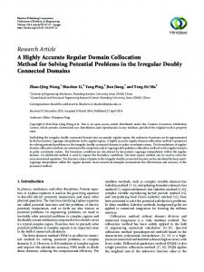
Figure 1: The results of the present method calculation for 𝜅 = 0.02, 0.04, 0.1, 0.2, and 0.5, in the order of height.

The authors are very grateful to the referees for their valuable suggestions and comments that improved the paper. Adem Kılıçman gratefully acknowledges that this research was partially supported by the University Putra Malaysia under the ERGS Grant Scheme having project number 5527068.

different step sizes, together with the results given in [23, 27– 29] and exact values

References

𝑢max = 1 + 𝜅 ln (

𝜅 ) 1 + 𝜅 − 𝑢0

(26)

reported in [21], are presented. Compared with other methods, our method provides more accurate numerical results. Note that the step sizes considered in Table 1 are based on the position of 𝑢max . To this end, for all values of 𝜅, we first solved the problem with the step size ℎ = 1 and 𝑁 = 15 to find the approximate position of 𝑢max . Then for each value of 𝜅 we selected an appropriate step size. Figure 1 shows the results of the present step by step collocation method for 𝜅 = 0.02, 0.04, 0.1, 0.2, and 0.5. This figure shows the rapid rise along the logistic curve followed by the slow exponential decay after reaching the maximum point, and when 𝜅 increases, the amplitude of 𝑢(𝑡) decreases whereas the exponential decay increases. Also, this figure shows the stability of the present method in large number of steps calculations.

4. Conclusion A new efficient step by step collocation method based on shifted Legendre-Gauss points has been proposed for solving Volterra model for population growth of a species in a closed system. We considered a step size and converted the original IVP raised from Volterra’s population model to a sequence of IVPs in subintervals and solved them, step by step, using collocation. This approach is easy to implement and possesses the spectral accuracy. Furthermore, this method is available for large domain calculations. Numerical example shows

[1] O. Coulaud, D. Funaro, and O. Kavian, “Laguerre spectral approximation of elliptic problems in exterior domains,” Computer Methods in Applied Mechanics and Engineering, vol. 80, no. 1–3, pp. 451–458, 1990. [2] D. Funaro, “Computational aspects of pseudospectral Laguerre approximations,” Applied Numerical Mathematics, vol. 6, no. 6, pp. 447–457, 1990. [3] J. Shen, “Stable and efficient spectral methods in unbounded domains using Laguerre functions,” SIAM Journal on Numerical Analysis, vol. 38, no. 4, pp. 1113–1133, 2000. [4] D. Funaro and O. Kavian, “Approximation of some diffusion evolution equations in unbounded domains by Hermite functions,” Mathematics of Computation, vol. 57, no. 196, pp. 597–619, 1991. [5] B.-Y. Guo, “Error estimation of Hermite spectral method for nonlinear partial differential equations,” Mathematics of Computation, vol. 68, no. 227, pp. 1067–1078, 1999. [6] C. I. Christov, “A complete orthonormal system of functions in 𝐿2 (∞, −∞) space,” SIAM Journal on Applied Mathematics, vol. 42, no. 6, pp. 1337–1344, 1982. [7] J. P. Boyd, “Spectral methods using rational basis functions on an infinite interval,” Journal of Computational Physics, vol. 69, no. 1, pp. 112–142, 1987. [8] J. P. Boyd, “Orthogonal rational functions on a semi-infinite interval,” Journal of Computational Physics, vol. 70, no. 1, pp. 63– 88, 1987. [9] B.-Y. Guo, J. Shen, and Z.-Q. Wang, “A rational approximation and its applications to differential equations on the half line,” Journal of Scientific Computing, vol. 15, no. 2, pp. 117–147, 2000. [10] J. P. Boyd, C. Rangan, and P. H. Bucksbaum, “Pseudospectral methods on a semi-infinite interval with application to the

6

[11]

[12]

[13]

[14]

[15]

[16]

[17] [18]

[19] [20] [21]

[22]

[23]

[24]

[25]

[26]

[27]

[28]

Mathematical Problems in Engineering hydrogen atom: a comparison of the mapped Fourier-sine method with Laguerre series and rational Chebyshev expansions,” Journal of Computational Physics, vol. 188, no. 1, pp. 56– 74, 2003. K. Parand, S. Abbasbandy, S. Kazem, and A. R. Rezaei, “Comparison between two common collocation approaches based on radial basis functions for the case of heat transfer equations arising in porous medium,” Communications in Nonlinear Science and Numerical Simulation, vol. 16, no. 3, pp. 1396–1407, 2011. C. E. Grosch and S. A. Orszag, “Numerical solution of problems in unbounded regions: coordinate transforms,” Journal of Computational Physics, vol. 25, no. 3, pp. 273–295, 1977. J. P. Boyd, “The optimization of convergence for Chebyshev polynomial methods in an unbounded domain,” Journal of Computational Physics, vol. 45, no. 1, pp. 43–79, 1982. B.-Y. Guo, “Jacobi spectral approximations to differential equations on the half line,” Journal of Computational Mathematics, vol. 18, no. 1, pp. 95–112, 2000. B.-y. Guo, “Jacobi approximations in certain Hilbert spaces and their applications to singular differential equations,” Journal of Mathematical Analysis and Applications, vol. 243, no. 2, pp. 373– 408, 2000. M. Maleki, I. Hashim, and S. Abbasbandy, “Analysis of IVPs and BVPs on semi-infinite domains via collocation methods,” Journal of Applied Mathematics, vol. 2012, Article ID 696574, 21 pages, 2012. J. P. Boyd, Chebyshev and Fourier Spectral Methods, Dover Publications, New York, NY, USA, 2nd edition, 2000. M. Maleki and M. Tavassoli Kajani, “A nonclassical collocation method for solving two-point boundary value problems over infinite intervals,” Australian Journal of Basic and Applied Sciences, vol. 5, no. 9, pp. 1045–1050, 2011. F. M. Scudo, “Vito Volterra and theoretical ecology,” Theoretical Population Biology, vol. 2, pp. 1–23, 1971. R. D. Small, Population Growth in a Closed System and mathematical Modelling, SIAM, Philadelphia, Pa, USA, 1989. K. G. TeBeest, “Numerical and analytical solutions of Volterra’s population model,” SIAM Review, vol. 39, no. 3, pp. 484–493, 1997. K. Al-Khaled, “Numerical approximations for population growth models,” Applied Mathematics and Computation, vol. 160, no. 3, pp. 865–873, 2005. A.-M. Wazwaz, “Analytical approximations and Padé approximants for Volterra’s population model,” Applied Mathematics and Computation, vol. 100, no. 1, pp. 13–25, 1999. K. Parand and M. Razzaghi, “Rational Chebyshev tau method for solving Volterra’s population model,” Applied Mathematics and Computation, vol. 149, no. 3, pp. 893–900, 2004. K. Parand and M. Razzaghi, “Rational Chebyshev tau method for solving higher-order ordinary differential equations,” International Journal of Computer Mathematics, vol. 81, no. 1, pp. 73– 80, 2004. K. Parand and M. Razzaghi, “Rational legendre approximation for solving some physical problems on semi-infinite intervals,” Physica Scripta, vol. 69, no. 5, pp. 353–357, 2004. M. Ramezani, M. Razzaghi, and M. Dehghan, “Composite spectral functions for solving Volterra’s population model,” Chaos, Solitons and Fractals, vol. 34, no. 2, pp. 588–593, 2007. H. R. Marzban, S. M. Hoseini, and M. Razzaghi, “Solution of Volterra’s population model via block-pulse functions and

Lagrange-interpolating polynomials,” Mathematical Methods in the Applied Sciences, vol. 32, no. 2, pp. 127–134, 2009. [29] K. Parand, A. R. Rezaei, and A. Taghavi, “Numerical approximations for population growth model by rational Chebyshev and Hermite functions collocation approach: a comparison,” Mathematical Methods in the Applied Sciences, vol. 33, no. 17, pp. 2076–2086, 2010. [30] N. A. Khan, A. Ara, and M. Jamil, “Approximations of the nonlinear Volterra’s population model by an efficient numerical method,” Mathematical Methods in the Applied Sciences, vol. 34, no. 14, pp. 1733–1738, 2011. [31] M. Abramowitz and I. Stegun, Handbook of Mathematical Functions with Formulas, Graphs, and Mathematical Tables, Dover Publications, New York, NY, USA, 1965.

Advances in

Operations Research Hindawi Publishing Corporation http://www.hindawi.com

Volume 2014

Advances in

Decision Sciences Hindawi Publishing Corporation http://www.hindawi.com

Volume 2014

Journal of

Applied Mathematics

Algebra

Hindawi Publishing Corporation http://www.hindawi.com


Volume 2014

Journal of

Probability and Statistics Volume 2014

The Scientific World Journal Hindawi Publishing Corporation http://www.hindawi.com


Volume 2014

International Journal of

Differential Equations Hindawi Publishing Corporation http://www.hindawi.com

Volume 2014

Volume 2014

Submit your manuscripts at http://www.hindawi.com International Journal of

Advances in

Combinatorics Hindawi Publishing Corporation http://www.hindawi.com

Mathematical Physics Hindawi Publishing Corporation http://www.hindawi.com

Volume 2014

Journal of

Complex Analysis Hindawi Publishing Corporation http://www.hindawi.com

Volume 2014

International Journal of Mathematics and Mathematical Sciences


Journal of

Mathematics Hindawi Publishing Corporation http://www.hindawi.com

Volume 2014


Volume 2014

Volume 2014


Volume 2014

Discrete Mathematics

Journal of

Volume 2014


Discrete Dynamics in Nature and Society

Journal of

Function Spaces Hindawi Publishing Corporation http://www.hindawi.com

Abstract and Applied Analysis

Volume 2014


Volume 2014


Volume 2014

International Journal of

Journal of

Stochastic Analysis

Optimization



Volume 2014

Volume 2014