applications may only be concerned with tidal effects while other may be heavily de- ...... MacBook with 2.4Ghz Core2Duo and 2GB of 1067 MHz DDR3 memory.
A Multiscale Framework for Bayesian Inference in Elliptic Problems by
Matthew David Parno B.S., Electrical Engineering, Clarkson University (2009) B.S., Applied Mathematics and Statistics, Clarkson University (2009) Submitted to the School of Engineering in partial fulfillment of the requirements for the degree of Master of Science in Computation for Design and Optimization at the MASSACHUSETTS INSTITUTE OF TECHNOLOGY June 2011 c Massachusetts Institute of Technology 2011. All rights reserved.
Author . . . . . . . . . . . . . . . . . . . . . . . . . . . . . . . . . . . . . . . . . . . . . . . . . . . . . . . . . . . . . . School of Engineering May 14, 2011 Certified by . . . . . . . . . . . . . . . . . . . . . . . . . . . . . . . . . . . . . . . . . . . . . . . . . . . . . . . . . . Youssef Marzouk Boeing Assistant Professor of Aeronautics and Astronautics Thesis Supervisor Accepted by . . . . . . . . . . . . . . . . . . . . . . . . . . . . . . . . . . . . . . . . . . . . . . . . . . . . . . . . . Nicolas Hadjiconstantinou Associate Professor of Mechanical Engineering Director, Computation for Design and Optimization
A Multiscale Framework for Bayesian Inference in Elliptic Problems by Matthew David Parno Submitted to the School of Engineering on May 14, 2011, in partial fulfillment of the requirements for the degree of Master of Science in Computation for Design and Optimization
Abstract The Bayesian approach to inference problems provides a systematic way of updating prior knowledge with data. A likelihood function involving a forward model of the problem is used to incorporate data into a posterior distribution. The standard method of sampling this distribution is Markov chain Monte Carlo which can become inefficient in high dimensions, wasting many evaluations of the likelihood function. In many applications the likelihood function involves the solution of a partial differential equation so the large number of evaluations required by Markov chain Monte Carlo can quickly become computationally intractable. This work aims to reduce the computational cost of sampling the posterior by introducing a multiscale framework for inference problems involving elliptic forward problems. Through the construction of a low dimensional prior on a coarse scale and the use of iterative conditioning technique the scales are decouples and efficient inference can proceed. This work considers nonlinear mappings from a fine scale to a coarse scale based on the Multiscale Finite Element Method. Permeability characterization is the primary focus but a discussion of other applications is also provided. After some theoretical justification, several test problems are shown that demonstrate the efficiency of the multiscale framework. Thesis Supervisor: Youssef Marzouk Title: Boeing Assistant Professor of Aeronautics and Astronautics
2
Acknowledgments I would not be where I am without Julie, who helps me keep things in perspective and maintain some sort of balance between work and play. I would also like to acknowledge the support of my parents; who have helped me stay on track and have pointed me towards quotes such as “Make friends with pain and you’ll never be alone,” from Ken Chlouber (founder of the Leadville 100) when I needed to dig deep. Of course my dad was talking about running the LeanHorse 100, but at times I think the same philosophy is useful in grad school. Additionally I would like to thank Sandia National Laboratories and the Office of Science Graduate fellowship for generous funding of this work.
3
Contents 0.1
Introduction . . . . . . . . . . . . . . . . . . . . . . . . . . . . . . . .
1 Inference Background 1.1
12 15
Deterministic Inversion Overview . . . . . . . . . . . . . . . . . . . .
15
1.1.1
Inverse Problem Formulation
. . . . . . . . . . . . . . . . . .
15
1.1.2
Optimization Approaches . . . . . . . . . . . . . . . . . . . .
17
1.2
Bayesian Inference Overview . . . . . . . . . . . . . . . . . . . . . . .
20
1.3
Bayes’ Rule . . . . . . . . . . . . . . . . . . . . . . . . . . . . . . . .
22
1.3.1
Brief History . . . . . . . . . . . . . . . . . . . . . . . . . . .
22
1.3.2
Derivation . . . . . . . . . . . . . . . . . . . . . . . . . . . . .
23
1.4
Bayesian Inference . . . . . . . . . . . . . . . . . . . . . . . . . . . .
24
1.5
Variational Bayes . . . . . . . . . . . . . . . . . . . . . . . . . . . . .
26
1.6
Sampling Methods . . . . . . . . . . . . . . . . . . . . . . . . . . . .
26
1.6.1
Rejection Sampling . . . . . . . . . . . . . . . . . . . . . . . .
27
1.6.2
Importance Sampling . . . . . . . . . . . . . . . . . . . . . . .
27
1.6.3
Markov chain Monte Carlo introduction . . . . . . . . . . . .
29
1.7
Dynamic Problems . . . . . . . . . . . . . . . . . . . . . . . . . . . .
34
1.8
Advanced MCMC . . . . . . . . . . . . . . . . . . . . . . . . . . . . .
35
1.8.1
Delayed Rejection Adaptive Metropolis MCMC . . . . . . . .
37
1.8.2
Langevin MCMC . . . . . . . . . . . . . . . . . . . . . . . . .
42
1.8.3
Other MCMC research . . . . . . . . . . . . . . . . . . . . . .
44
Inference Summary . . . . . . . . . . . . . . . . . . . . . . . . . . . .
45
1.9
4
2 Multiscale Background 2.1
2.2
46
Multiscale Simulation Methods . . . . . . . . . . . . . . . . . . . . .
48
2.1.1
Model Elliptic Equation . . . . . . . . . . . . . . . . . . . . .
48
2.1.2
Upscaling . . . . . . . . . . . . . . . . . . . . . . . . . . . . .
52
2.1.3
Homogenization . . . . . . . . . . . . . . . . . . . . . . . . . .
55
2.1.4
Variational Methods . . . . . . . . . . . . . . . . . . . . . . .
58
2.1.5
Multiscale Finite Element Methods . . . . . . . . . . . . . . .
59
Multiscale Sampling methods . . . . . . . . . . . . . . . . . . . . . .
63
2.2.1
Coupled Metropolis Sampling . . . . . . . . . . . . . . . . . .
63
2.2.2
Proposal Filtering with MsFEM . . . . . . . . . . . . . . . . .
65
3 Multiscale inference framework
67
3.1
Conditional Independence . . . . . . . . . . . . . . . . . . . . . . . .
67
3.2
Multiscale MCMC formulation . . . . . . . . . . . . . . . . . . . . . .
70
3.3
Upscaling the Prior . . . . . . . . . . . . . . . . . . . . . . . . . . . .
71
3.3.1
Proof of positive definiteness in one dimension . . . . . . . . .
77
Iterative Nonlinear Conditioning . . . . . . . . . . . . . . . . . . . . .
79
3.4.1
Linear conditioning . . . . . . . . . . . . . . . . . . . . . . . .
80
3.4.2
Nonlinear conditioning . . . . . . . . . . . . . . . . . . . . . .
82
3.4.3
MCMC along a constraint . . . . . . . . . . . . . . . . . . . .
89
3.5
Multiscale framework overview . . . . . . . . . . . . . . . . . . . . . .
91
3.6
Implementation details . . . . . . . . . . . . . . . . . . . . . . . . . .
92
3.6.1
Jacobian in One Dimension . . . . . . . . . . . . . . . . . . .
92
3.6.2
Other notes . . . . . . . . . . . . . . . . . . . . . . . . . . . .
93
Generalization to other multiscale settings . . . . . . . . . . . . . . .
93
3.4
3.7
4 Numerical Results 4.1
94
Test Cases . . . . . . . . . . . . . . . . . . . . . . . . . . . . . . . . .
94
4.1.1
Problem Description . . . . . . . . . . . . . . . . . . . . . . .
94
4.1.2
Verification with single scale inference results
96
4.1.3
Draw from Exponential Prior . . . . . . . . . . . . . . . . . . 100 5
. . . . . . . . .
4.1.4
First layer of SPE10 . . . . . . . . . . . . . . . . . . . . . . . 102
4.1.5
Fifth layer of SPE10 . . . . . . . . . . . . . . . . . . . . . . . 103
4.1.6
Summary of test cases . . . . . . . . . . . . . . . . . . . . . . 104
5 Future work and conclusions
5.1
106
5.0.7
Future work . . . . . . . . . . . . . . . . . . . . . . . . . . . . 106
5.0.8
Use in dynamic problems . . . . . . . . . . . . . . . . . . . . . 106
5.0.9
Spatial decoupling during iterative conditioning . . . . . . . . 107
Finale . . . . . . . . . . . . . . . . . . . . . . . . . . . . . . . . . . . 107
A Philosophical Asides
109
A.1 Epistemic and Aleatory Uncertainty . . . . . . . . . . . . . . . . . . . 109 A.2 Bayesian vs. Frequentist . . . . . . . . . . . . . . . . . . . . . . . . . 110
6
List of Figures 1-1 The danger of simply using a point estimate for the calibrated parameters. In the blue, noise in the data will not result in a large error in the calibrated model. However, the same amount of noise in the red could result in a calibrated parameter somewhere in the range of [−1.6, 1.6]. A Bayesian approach allows this uncertainty to be captured and presented as part of the final inference result. . . . . . . . . . . .
21
1-2 The likelihood function constrains the likely regions of the parameter space. When the error is large, i.e. γ is large for Σ�� = γI, the likelihood functions does not provide much new information and the posterior will be largely governed by the prior. . . . . . . . . . . . . .
25
1-3 Illustration of rejection sampling. Samples of the green distribution are generated by sampling from a distribution proportional to the red function (Gaussian in this case) and accepting with the probability defined in (1.17) . . . . . . . . . . . . . . . . . . . . . . . . . . . . . .
28
1-4 Example of a three state discrete Markov chain with transition probabilities denoted by pij . If you squint hard enough you can imagine a similar system in, IRm , where we have an infinite number of states. . .
31
1-5 Example of Metropolis-Hastings MCMC sampling a simple Gaussian mixture in 2 dimensions. Shown is the MCMC chain after 50 iterations, the density estimate after 10000 steps, and the chain after 2000 steps.
33
1-6 Example of Metropolis-Hastings samples for increasing proposal variance. The contours show the true distribution, which has a mean of (0, −2).
. . . . . . . . . . . . . . . . . . . . . . . . . . . . . . . . . . 7
37
1-7 Example of Metropolis-Hastings chains for increasing proposal variance. Blue is the x component of the chain and green is the y component. For small proposals, high acceptance rates exist but the jumps are small and the chain inefficiently explores the space (the meandering nature in the first plot). However, for too large a proposal, the frequent plateaus indicate that the acceptance probability is low. . . .
38
1-8 Comparison of the DRAM family of adaptive algorithms. Blue is the x component of the chain and green is the y component. The initial proposal size was set to C0 = 2I. Three DR stages were used, each shrinking the previous proposal by a factor of 4. The covariance was adapted with AM every 20 steps. . . . . . . . . . . . . . . . . . . . .
42
2-1 Example of groundwater observations with multiscale behavior. Not only are yearly patterns present, but daily length scales exist as well. Data comes from USGS well measurements in Bingham County, Idaho. 47 2-2 Conservation of mass in a porous media. When coupled with Darcy’s equation as a constitutive law, this gives the familiar pressure equation. 48 2-3 Example of multiscale field and corresponding pressures. The one dimensional case has a dirichlet condition on the left and a homogeneous Neumann condition on the right. In the two dimensional case, all boundaries are fixed with Dirichlet conditions. Clearly, the pressure fields are much smoother than the permeability fields. The one dimensional case shows the smoothing effect of the elliptic operator and the two dimensional setting again shows the relative smoothness of the pressure field compared to the permeability field. . . . . . . . . . . .
51
2-4 Example of geometric, arithmetic, and harmonic averaging. After inspection, note that the geometric means visually seems to be between the arithmetic and harmonic means, as required by the Wiener bounds. This field is log10 (K) for the 10th layer of the popular SPE10 dataset.
8
54
2-5 Comparison of Homogenization process and upscaling process. While upscaling builds a coarse permeability and uses the same governing equation, homogenization finds a homogenized permeability by putting constraints on the coarse operator. . . . . . . . . . . . . . . . . . . .
56
2-6 Illustration of MsFEM Basis function. This illustrates the basis function evaluated over one coarse element. . . . . . . . . . . . . . . . . .
61
2-7 Illustration of the Multiscale Metropolis MCMC method. Here, steps labeled with MCMC correspond to steps with standard single scale proposals. It is also possible to have more than one MCMC step before a swap is performed. . . . . . . . . . . . . . . . . . . . . . . . . . . .
64
3-1 Validation of conditional independence assumption. . . . . . . . . . .
69
3-2 Illustration of full multiscale inference using procedure using MsFEM.
71
3-3 Quantile-Quantile plot comparing sample quantiles to true log-normal quantiles. The distribution is an exact fit when the scatter points are exactly linear. . . . . . . . . . . . . . . . . . . . . . . . . . . . . . . .
74
3-4 Distribution of log(e) based on Monte-Carlo sampling of a piecewise constant log-normal k field with exponential prior. . . . . . . . . . . .
75
3-5 Distribution of log(e) based on Monte-Carlo sampling of a piecewise constant log-normal k field with Gaussian prior. . . . . . . . . . . . .
76
3-6 Mapping from π(Y ) to π(log(e)) for exponential and Gaussian covariance kernels in π(Y ). The fine scale correlation length, Lf , has been scaled by the coarse element size h to allow for arbitrary discretizations. Notice the x axis of the power plots is in the opposite direction to the other plots. . . . . . . . . . . . . . . . . . . . . . . . . . . . . .
78
3-7 Illustration of π(k|A) as a constraint on the prior. We wish to sample from the “slice” of π(k) along the constraint. . . . . . . . . . . . . . .
80
3-8 Comparison of high order ODE integration with SCKF for sampling from a constraint. The densities are plotted over x. . . . . . . . . . .
9
86
3-9 Illustration of integration paths for nonlinear conditioning and linear conditioning . . . . . . . . . . . . . . . . . . . . . . . . . . . . . . . .
88
3-10 Illustration of conditioned proposals in two dimensions on a cubic constraint. In both cases, λ = 0.01. . . . . . . . . . . . . . . . . . . . . .
91
4-1 Location of pressure observations and posterior covariance comparison using the fully multiscale approach, single scale with FEM forward solver, and single scale with MsFEM forward simulation. . . . . . . .
97
4-2 Comparison of posterior mean and variance between standard single scale approaches and the multiscale framework. The left plot shows the posterior means ±2σ 2 . . . . . . . . . . . . . . . . . . . . . . . .
98
4-3 Results for multiscale inference using a draw from the prior. The prior kernel is defined by p = 1, d = 0.2, σ = 1. Twenty fine elements were used in each coarse element and 5 coarse elements were used. . . . . . 101 4-4 Results for multiscale inference using a slice of layer 1 of the SPE 10 datset. The chain was downsampled by 50 before iterative conditioning.103 4-5 Results for multiscale inference using a slice of layer 5 of the SPE 10 datset. The chain was downsampled by 50 before iterative conditioning.105
10
List of Tables 1.1
Example of Metropolis-Hastings MCMC performance on two dimensional Banana function. Proposal is diagonal Gaussian. 100 trials with 1000 Samples after a burn in period of 200 steps was used. . . . . . .
3.1
36
Comparison of acceptance rates for MCMC on cubic constraint with � = 1e − 2. The bold rates are the combinations that result in the smallest density reconstruction error from 500 nonlinear conditioning runs and 500 MCMC steps. . . . . . . . . . . . . . . . . . . . . . . .
4.1
91
Comparison of single scale performance with multiscale performance. ESS is the effective sample size, so ESS/N is the effective number of samples related to the total number of fine scale samples generated and ESS/S is the number of effective samples per second. . . . . . .
4.2
99
Summary of multiscale inference tests. Kc is the number of coarse elements, Kf is the number of fine elements in each coarse element. d is the correlation length of the prior, p is the prior power, σ is the prior variance, µY is the prior mean, Nd is the number of data points. . . . 100
4.3
Summary of multiscale inference performance. ESS is the effective sample size, so ESS/N is the effective number of samples related to the total number of fine scale samples generated and ESS/S is the number of effective samples per second. Additionally, acceptance is the acceptance rate of the coarse MCMC chain. . . . . . . . . . . . . 104
11
0.1
Introduction
Humans have been trying to understand the world around us for millennia. Take for example the Babylonian mathematicians around 1700 BCE, who put together a tablet of Pythagorean triples [1]. Obviously, we are now far beyond the computing power of a few mathematicians with clay tablets and a base 60 number system. With the advent of computers, our predictive capabilities have increased dramatically. We can now perform simulations on huge supercomputers or large distributed systems to simulate large fusion reactors [74] or protein folding in a cell [6]. Advanced simulations like these and even much less sophisticated mathematical models serve two purposes: the model allows scientists and engineers to make predictions about how a system behaves and the model gives insight into why the system behaves as it does. For example, modeling glacier dynamics is important not only for predicting human influence on the environment [13] but also to help researchers answer fundamental questions about why glaciers behave the way they do [57]. However, nearly all models contain at least a few tunable parameters or parameter fields that are not known exactly. The parameters considered here usually represent physical characteristics of the system being simulated. Examples include chemical reaction rates in combustion simulations and permeability fields in groundwater models. Regardless of the physical situation, it is usually necessary to tune model parameters to ensure model predictions agree with physical observations. Accurate calibration is critical for informative predictions. Additionally, in some situations, finding suitable parameters is the end goal. In order to understand the mechanics of glacier flow, glaciologists need to find basal stresses under a glacier. Obviously these cannot be measured directly, but their effect on glacial motion can be modeled. Thus, finding basal stresses is the end goal; future simulations using these values is a secondary objective. In practice, there is usual some error in observational data, and as the glaciology example shows, available observations may be indirect. The fundamental problem here of using noisy observations to find appropriate parameter values is usually called an inference problem, inverse problem, calibration problem,
12
or parameter estimation problem. The rest of this chapter will describe many of the existing methods for parameter estimation, which can be quite costly for large scale problems. To reduce the computational complexity, chapter 3 will introduce multiscale techniques for simulating groundwater flow. The application of these techniques in solving the inference problem will then be discussed. It will be shown that multiscale concepts can be used when solving an inference problem to dramatically reduce the required computational effort. The final chapter will discuss the performance of the multiscale procedure on a variety of test problems. Historically, computational restrictions have forced simulation based engineering analysis and design to use deterministic methods. However, input data to numerical simulations are rarely known exactly in real engineering problems and understanding uncertainties in numerical predictions is paramount to creating robust designs. With the recent explosion of computational resources, there has been significant work towards efficiently characterizing the uncertainty in numerical predictions, especially in the context of large partial differential equation based mathematical models. In most cases, the uncertainty in these problems comes from incomplete knowledge of a model parameter or field. In a hydrology setting, the uncertain field is often subsurface permeability. The permeability field is rarely known precisely and forward uncertainty quantification methods are required to characterize model predictions of pressure, saturation, etc... Before these forward predictions can be used in engineering analysis, a probabilistic description of the field should be constructed from any available information. That is, an inference problem needs to be solved before the model can be used for prediction. Mathematically, an inverse problem is to find parameters k based on limited data d and a function G(k) that maps the parameter to a predicted ˜ d: d˜ = G(k)
(1)
Because G(k) usually depends on a simulation or model of the physical system generating d, we cannot hope to fully capture all the physics and processes that generated d. The prediction d˜ is only expected to approximately represent the potentially noisy
13
data d. Adding an error term, � is one approach to incorporate this approximation: d = G(k) + �
(2)
This is an example of an additive error model. This choice is not unique, multiplicative error models are also common. In that case, d = (1 + �)G(k)
(3)
Other error models are also used depending on the specific application. Specifically, the error model can be tailored to acknowledge unmodeled physics or systematic measurement error. In this work, the additive error model will be used. However, all of many methods presented throughout this text can also be applied to situations with more sophisticated error models. Authors will often cite two classes of uncertainty that go into �: epistemic uncertainty and aleatoric uncertainty. No distinction between the two will be made here because I feel in the macroscale PDE setting studied here, the distinction is superfluous. An interested reader should refer to appendix A.1 for a detailed discussion.
14
The only source of knowledge is experience. Albert Einstein
Chapter 1 Inference Background 1.1 1.1.1
Deterministic Inversion Overview Inverse Problem Formulation
Let k be a finite dimensional model parameter. The problem of characterizing k from limited data d can be rephrased as finding an estimate k ∗ that minimizes the difference between G(k) and d. The simplest and probably most well known approach is to find k that minimizes the L2 error: k ∗ = argmin kG(k) − dk22 = argmin (G(k) − d)T (G(k) − d) k
(1.1)
k
which is simply nonlinear least squares. Various forms of nonlinear least squares, often with some sort of regularization, remain the standard formulation of deterministic inversion. A slightly more general weighted form is often used: k ∗ = argmin (G(k) − d)T W (G(k) − d)
(1.2)
k
where W is some weighting matrix representing the differences in measurement error or importance of each piece of data. In instances where the dimension of d is less than the dimension of k, or when large variations in k cause relatively small changes in G(k), the inverse problem can become underdetermined or ill-posed and many 15
different values of k will give nearly identical objective values. The study of such ill-posed problems really begins with Hadamard in 1902. He was the first person to formally define what it means for a problem to be well posed, or “un probl`em bien pos´e” in the original paper, [37]. There he states that a problem is well posed if the following three conditions are satisfied: • The solution, k ∗ , exists • The solution, k ∗ , is unique • The solution, k ∗ , is stable Here, stability implies the solution k ∗ depends continuously on the data. When any one of these conditions is not satisfied, the problem is called ill-posed. Being primarily concerned with under determined problems in this text, the condition that the inverse problem solution be unique is our primary concern. Much of the work in inverse problems can be interpreted as attempts to transform an ill-posed problem to into “un probl`em bien pos´e” by modifying the formulation. Additional work then focuses on efficient solution methods. In order to ensure a uniquely solvable problem, more information needs to be used in the optimization problem formulation. A standard methodology introduced by Tikhonov in [76] and now widely used to solve ill-posed problems, is to add a regularization term to the objective, resulting in k ∗ = argmin (G(k) − d)T W (G(K) − d) + k T (ΓT Γ)k
(1.3)
k
where Γ is called the Tikhonov matrix. When Γ is properly chosen, the added regularization problem ensures the well-posedness of the problem. This new problem is sometimes called a damped least squares problem. Choosing the Tikhonov matrix is important for efficiently solving the problem with a nonlinear optimization technique. More information on choosing Γ can be found in [4] , where a general discussion of least squares methods is given. Tikhonov regularization is also used in the well known software package (PEST) developed by John Doherty for calibration problems arising 16
in subsurface flow. The PEST manual, [14], provides a description of nonlinear least squares with Tikhonov regularization in a practical setting. The introduction of the Tikhonov penalty term can also be motivated through the Bayesian paradigm. This will be discussed in more detail in later sections; however, the interested reader should note that Γ is related to the Bayesian prior distribution for k. Compressive sensing techniques in the image and signal processing literature can also be viewed as a regularization to combat ill-posedness. In those problems, a limited number of samples are used to reconstruct a signal or image in a large dimensional space. In that setting, the number of nonzero terms in k is used as a penalty to regularize the system. See [11] for an introduction to this topic.
1.1.2
Optimization Approaches
Solving the formulation in (1.3) can be difficult in real-world applications where G(k) is a highly nonlinear model, and the data d have significant noise. The speed of Newton’s method makes it the usual first choice for optimization algorithms, when Hessian information is available. However, obtaining accurate Hessians to (1.3) is infeasible in most real problems. Thus, Quasi-Newton methods that approximate the Hessian are often used. Standard Quasi-Newton methods for nonlinear least squares are the Gauss-Newton and the related Levenberg-Marquadt algorithms. These methods use the Jacobian of G(k) and the residual to find an approximate Newton descent direction. First, define the residual vector, r(k) as: r(k) = (G(k) − d)
(1.4)
Now, the original weighted least squares problem in (1.2) can be rewritten as k ∗ = argmin r(k)T W r(k) k
17
(1.5)
Clearly, the residual is nonlinear in k because of the nonlinear forward model G(k). Thus, linearizing r(k) about a point k − gives: r(k) ≈ r(k − ) + J(k − )(k − k − )
(1.6)
where J(k − ) is the Jacobian matrix of G(k) at k − . Using this approximation in the least squares problem, we have: � �T � � r(k)T W r(k) ≈ r(k − ) + J(k − )(k − k − ) W r(k − ) + J(k − )(k − k − )
(1.7)
which is simply a linear weighted least squares problem. The solution, k + to this is just a solution to the normal equations and can be written as: �−1
� � W J Jk − − r(k − ) �−1 = k− − J T W J W Jr(k − )
k+ =
JT W J
(1.8)
where the dependence of the Jacobian on k − was dropped for clarity of expression. The Gauss-Newton method will use k + as the next step in an iterative process that builds this linear approximation and solves the resulting linear least squares problem at each step. Compare (1.8) with the iteration in Newton’s method: � k + = k − − H −1 ∇ r(k − )T W r(k − ) = k − − H −1 W Jr(k − )
(1.9)
Clearly, the Gauss-Newton method is Newton’s method with an approximate Hessian given by J T W J. In fact, another derivation of the Gauss-Newton algorithm given in [52], obtains the Gauss-Newton step simply by looking at a Taylor approximation of the Hessian. To apply the Gauss-Newton method, the matrix J T W J needs to be nonsingular and well conditioned. This can be quite limiting in practice. [52]. The Levenberg-Marquadt algorithm addresses this issue by introducing a regularization
18
paraemter, λ to (1.8), resulting in: k + = k − + J T W J + λI
�−1
� � W J G(k − ) − d
(1.10)
Combined with a line search and adaptation strategy for λ, this can perform quite well even when starting far from a local minima. Adapting the regularization parameter λ so that λ → 0 as k + → k ∗ , as in PEST, [14], allows the Levenberg-Marquadt method to recover the speed of the Gauss-Newton algorithm in a basin of attraction around the optimum. It should also be noted that the Levenberg-Marquadt algorithm can be interpreted as Gauss-Newton with a trust region, so near the optimum, the trust region is large and does not restrict the step, resulting in pure Gauss-Newton iterations. See [52] for a rigorous discussion on the convergence of these methods. In addition to these classical methods, there has also been some recent work in [9] and [10] using preconditioned Newton-Krylov methods for largescale PDE-constrained optimization problems. These methods use a very sophisticated adaptation of Newton’s method to address the problem of inverse problems when the underlying partial differential equations are known. The classical methods above require Jacobian information and the work of Biros and Ghattas in [9, 10] requires Hessian information. In some instances adjoint methods can be used to efficiently obtain this higher order information and these derivative based methods can be used. In addition to [9, 10] examples using adjoints can be found in glacial dynamics calibration, [63]. A control theoretic approach using adjoints is often implemented in the glaciology community to infer basal boundary conditions [63, 49]. Additional information on adjoint methods for largescale optimization can be found in [8]. Unfortunately, for many intriguing calibration problems, adjoints are not a viable option due to complicated models or black box simulations. While the naive approach would be to use finite difference approximations1 , derivative free optimization tools are a significantly more efficient option. Varying from simple pattern search methods to sophisticated hybrid algorithms, there is no clear winner 1
This is in what PEST does by default
19
when it comes to derivative free techniques; however, comparison papers such [62, 25] and application papers such as [58, 40] give guidance for choosing a derivative free algorithm.
1.2
Bayesian Inference Overview
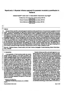
In its simplest form, deterministic inversion gives a single point estimate for the calibrated parameters. Noisy data and approximate models bring into question how useful the parameter estimate will be for future predictions. Some deterministic methods can use Hessian information at the optimum to approximate local covariance but in nonlinear problems this approximation does not adequately quantify uncertainty in the solution.2 Figure 1-1 illustrates in a simple setting the large effect that unquantified noise can have on a parameter estimate. The solid lines are illustrations of the least squares objective function and the the dashed lines show some uncertainty in the objective values coming from noise in the data. Deterministic inversion ignores the error and would only minimize the solid lines. In the blue case, there is a sharp valley and any objective within the dashed lines would produce a similar least squares estimate for k. An objective like this could occur for a hyperbolic or nearly hyperbolic PDE forward model where k could be an initial condition. On the other hand, the red line has a much broader valley, perhaps coming from an elliptic or parabolic PDE model where the data is from a much smoother field than the parameter k. In the wider case, within the dashed lines the least squares estimate for k could be in a wide range ≈ [−1.7, 1.7]. However, without incorporating the data noise into the parameter estimation problem problem, a deterministic least squares estimate would give k = 0 for both systems and a user would have no idea how reliable a forward prediction with the estimated k will be. This can be particularly troublesome when estimating a parameter from smooth data, such as pressure data 2
For a linear model using Gaussian random variables in a Bayesian formulation, the inverse of the Hessian corresponds to the posterior covariance. In nonlinear models or non Gaussian distributions, the posterior distribution will not be Gaussian and cannot be completely described by a point estimate and covariance matrix.
20
1.2 1
kG(k) − dk22
0.8 0.6 0.4 0.2 0 −0.2 −6
−4
−2
0 k
2
4
Figure 1-1: The danger of simply using a point estimate for the calibrated parameters. In the blue, noise in the data will not result in a large error in the calibrated model. However, the same amount of noise in the red could result in a calibrated parameter somewhere in the range of [−1.6, 1.6]. A Bayesian approach allows this uncertainty to be captured and presented as part of the final inference result. in a hydrology context, and then using that estimate in a hyperbolic system, such as tracer transport. Variability in the parameter estimate is dissipated by an elliptic operator, but when used in a hyperbolic operator, the forward predictions could be far from the truth. Bayesian inference is a probabilistic tool that allows uncertainty to be represented during the entire inference process. The goal is to build a probability density for k that is conditioned on the data. Before proceeding, it is important to note that in many senses, Bayesian methods can be interpreted as generalization of more commonly used frequentist methods. Sec A.2 in the appendix provides a brief justification for the Bayesian interpretation as a useful alternative to frequentist interpretations.
21
1.3
Bayes’ Rule
In addition to the derivation below, good introductions to Bayesian inference and Bayes’ can be found in [70, 29, 51]. However, a much more thorough discussion using manifolds is given in [75]. The latter approach allows for nonlinear data and model spaces which are not considered here. Additionally, [75] and [51] give a discussion on the Bayesian interpretation of least-squares problems.
1.3.1
Brief History
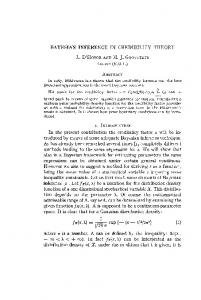
In words, Bayes’ rule (often called Bayes’ theorem) updates a prior belief of a parameter’s value with data to create a posterior belief. The degrees of belief are quantified with probability distributions. Reverand Thomas Bayes first introduced his theorem3 in the 18th century with application to the Binomial distribution. It was then generalized to arbitrary distributions by Laplace.4 However, Laplace limited his choice of prior distribution to uniform distributions. After some controversy and friction between frequentists and Bayesians (see appendix A.2 for more information), in the early 20th century, the works of Harold Jeffrey’s and Edwin Jaynes pushed Bayesian inference into the mainstream. Good textbooks by these authors can be found in [46] and [45]. As pointed out in [68], the widespread adoption of Markov chain Monte Carlo (MCMC) methods in the Bayesian setting did not occur until the late 1980s or early 1990s. The application of MCMC to sampling of posterior distributions, helped launch Bayesian statistics towards reall applications and approach its current state as a general inference framework. 3
Bayes in fact did not publish his work, his friend Richard Price actually published Bayes’ work after his death. Interestingly, Richard Price thought that Bayes’ theorem could help prove the existence of god. See [5] for the original letter by Price accompanying the original essay by Bayes. 4 Laplace actually reinvented Bayes’ rule from scratch and showed its use for general densities, it was only later that he discovered the original work of Bayes
22
1.3.2
Derivation
In its modern presentation, Bayes’ rule relies on the ideas of conditional probability and the interpretation of a probability as a degree of belief. Define a probability space (Ω, U, µ), where Ω is the sample space, U is a σ-algebra defined on Ω and µ is a probability measure on U . A usual choice of U is the Borel σ-algebra. Any subset, A ⊂ U , is called an event, so U represents all events that could occur. In the inference setting, U is all sufficiently well behaved sets of k. The probability of an event occurring is computed from the probability measure as: Z dµ(ω)
P (A) =
(1.11)
A
for ω ∈ Ω. Note that several probability measures can be defined over U . This is in fact how degrees of belief will be defined. The prior degree of belief will be defined as a prior measure on U and the posterior degree of belief will be defined as a posterior measure on U . The remainder of this text deals exclusively with real valued random variables, so we will assume µ has a density π with respect to Lebesgue measure. Now, let k be the parameter of interest and d be available data. The goal is to find the density π(k|d). Using the law of total probability this can be rewritten as πk|d (k|d) =
πk,d (k, d) πd (d)
Expanding the joint distribution in the other order gives: πk|d (k|d) =
πd|k (d|k)πk (k) πd (d)
Now rewriting the denominator: πd|k (d|k)πk (k) π (d|k)πk (k)dk U d|k
πk|d (k|d) = R
(1.12)
Since the denominator does not depend on k, it is not required during inference5 and 5
The denominator, called the evidence is not needed during inference but is a critical quantity
23
(1.12) is usually written more compactly as: πk|d (k|d) ∝ πd|k (d|k)πk (k)
(1.13)
which is the familiar Bayes’ rule of conditioning. The prior density, hereafter just referred to as the prior, is πk (k) and the posterior is πk|d (k|d). Additionally, πd|k (d|k) is referred to as the likelihood function or just likelihood. The likelihood is usually chosen to be of a particular form based on the noise in d. The difficulty in Bayesian inference methods is how to characterize πk|d (k|d). In practical applications, the posterior can rarely be expressed in an analytic form and needs to be approximated numerically.
1.4
Bayesian Inference
As in the deterministic setting, denote the forward model parameterized by k as G(k). Incorporating a similar error, d = G(k) + �
(1.14)
where we will assume � ∼ N (0, Σ�� ). The distribution of � is called the error model. While an additive Gaussian error model is used here, applications with more systematic error exist and will generally use non-additive and/or non-Gaussian error models. For example, in signal processing much of the noise comes from other communication systems and has more structure than the simple additive Gaussian model used. In that situation more suitable error models exist, see [60] for more information on general noise models in the signal processing context. In the additive Gaussian error case, the likelihood is given by: � � 1 T −1 πd|k (d|k) = p exp − (G(k) − d) Σ�� (G(k) − d) 2 (2π)k |Σ�� | 1
(1.15)
Evaluating G(k) may require solving a partial differential equation or calling a black in model comparison and Bayesian experimental design
24
15
15
10
10
5
5
G(k) 0
G(k) 0
−5
−5
−10
−10
−15 −2 −1.5 −1 −0.5
0
0.5
1
1.5
−2 −1.5 −1 −0.5
2
k 15
10
10
5
5
G(k) 0
G(k) 0
−5
−5
−10
−10
−2 −1.5 −1 −0.5
G(k) = d + �med 0
0
0.5
1
1.5
2
k
15
−15
G(k) = d + �small
−15
G(k) = d
0.5
1
1.5
G(k) = d + �large
−15 2
k
−2 −1.5 −1 −0.5
0
0.5
1
1.5
2
k
Figure 1-2: The likelihood function constrains the likely regions of the parameter space. When the error is large, i.e. γ is large for Σ�� = γI, the likelihood functions does not provide much new information and the posterior will be largely governed by the prior. box model where no analytical form exists for the likelihood. However, given a particular k, the likelihood can be evaluated and the posterior can then be evaluated. The likelihood functions acts as a weighting of the prior measure that ensures the posterior will respect the data. Therefore, when the data is extremely noisy, it is easier for a prediction to “agree” with the data and the posterior will be more similar to prior than if little noise was present. Figure 1-2 shows the effect of noise on a potential likelihood function. As more noise is added, more portions of the parameter space have significant probability and the prior begins to play a larger role. This has an interesting analogy with Tikhonov regularization. As the problem becomes more ill-posed in the Hadamard sense, the regularization term plays a more important role in the optimization. As will be shown later in section 1.6.3, even though the posterior density does
25
not have an analytic form, samples can still be drawn from the posterior distribution. These samples can then be used as an approximation to the posterior for use in future computations. While sampling methods are the focus of this work, it is important to note that alternatives exist. A variational approximation to the posterior can also be found.
1.5
Variational Bayes
The idea behind variational Bayesian methods is to approximate the posterior, πk|d (k|d) by a different parametric distribution π ˜θ (k; θ) by choosing θ to minimize the KullbackLeibler divergence between πk|d (k|d) and π ˜θ (k; θ). Formally, we have ∗
Z
θ = argmin
π ˜θ (k; θ) log U
π ˜θ (k; θ) dk πk|d (k|d)
(1.16)
The approximate distribution π ˜θ (k; θ) is usually composed of exponential families or another analytically tractable distributions. This is similar to finding the basis function coefficients that minimize the energy norm in finite element methods. For a more thorough introduction to variational Bayesian approaches, [55] provides an introductory chapter.
1.6
Sampling Methods
Given a sufficient number of samples from a distribution, any required statistic can be computed. This includes event probabilities and distribution moments. Sampling methods are designed to generate samples of a distribution for use in this type of calculation. There are a variety of sampling methods, each with its own niche in Bayesian analysis. However, Markov chain Monte Carlo (MCMC) methods are predominantly used in the inference setting described above. To contrast MCMC with other sampling approaches, this section gives an overview of a few popular methods. The number of methods is incredibly large, the methods described here are only meant to give a flavor of the field. More detailed information can be found in [29] 26
or [51]. Additionally, [67] and [54] provide more detailed discussions of Monte Carlo methods in general.
1.6.1
Rejection Sampling
Rejection sampling is a simple way to sample from an arbitrary distribution in any dimension. However, the emptiness of high dimensional spaces causes the method to become inefficient even for moderately sized problems. Suppose that we wish to generate samples from a general distribution with density π(k); however, we cannot directly from π(k). Introduce an alternative, easy to sample, density q(x). To generate a sample of π(k), we can first sample, k 0 from q(k) and accept this sample as a sample of π(k) with probability:
Paccept =
π(k 0 )/q(k 0 ) c
(1.17)
where c is the maximum ratio between the distributions: c = max k
π(k) q(k)
Figure 1-3 illustrates the rejection sampling process. The numerator of (1.17) in the figure is given by β/α. The normalization ensures the acceptance probability is always less than one.
1.6.2
Importance Sampling
Consider the problem of estimating the expectation of f (x) over the distribution π(x). That is, we wish to estimate Z Eπ [f (x)] =
Z f (x)dπ(x) =
27
f (x)π(x)dx
α β q(k) k0
π(k)
Figure 1-3: Illustration of rejection sampling. Samples of the green distribution are generated by sampling from a distribution proportional to the red function (Gaussian in this case) and accepting with the probability defined in (1.17) Instead of sampling from π(x) directly, we can sample from an alternative distribution q(x) and estimate the expectation as: Z Dπ [f (x)] =
f (x)
π(x) q(x)dx q(x)
N 1 X π(xi ) ≈ f (xi ) N i=1 q(xi )
where N is the number of samples and the xi are iid samples taken from the distribution q(·). Introducing the weights, w(xi ) =
π(xi ) , q(xi )
the approximate expectation is sim-
ply a sum of weighted samples. In standard Monte Carlo estimates, w(xi ) = 1. Now, instead of needing to pull samples from π(x) which may not be possible when π(x) is a complicated distribution, only samples of q(x) are needed. To make importance sampling worthwhile, q(x) is usually chosen from an easily sampleable distribution such as a Gaussian. Another desirable feature of importance sampling is that the weights, wi , also define the normalization factor in Bayes’ rule with no additional work. Let π(x) =
πd|k (d|k)πk (k) z
28
then, Z z=
πd|k (d|k)πk (k) q(x)dx q(x) N 1 X i ≈ w N i=1 Z
πd|k (d|k)πk (k)dx =
While this is a useful aspect of importance sampling, the choice of q(x) is not always obvious. Usually the distribution should approximate π(x) in some way, but π(x) could depend on the solution of PDE and be difficult to approximate. Also important i h π(x) for effective implementation is the weight variance, var q(x) . A small variance means the weights are approximately constant and therefore imply q(x) is a relatively good h i approximation to π(x). Alternatively, var π(x) could be used as a metric of the q(x) proposal efficiency. In fact, minimizing this variance produces the optimal q(x) in terms of reducing the estimate variance. The goal is then to find a q(x) that is in some sense close to the optimal proposal to minimize the weight variance; this will increase the method’s sampling efficiency. In some applications outside of inference, such as estimating the probability of rare events, importance sampling is currently the only feasible approach. Importance sampling allows a user to push sample points into very low probability regions that would otherwise go unsampled. This is advantageous when trying to accurately compute the probability of an event with small probability. In the rare event case, standard Monte Carlo sampling would waste many samples in high probability regions without gaining any information about the event of interest.
1.6.3
Markov chain Monte Carlo introduction
The difficulty in using importance sampling or rejection sampling to estimate distributionwide quantities is that high dimensional parameter spaces are quite empty, and these methods can waste a lot of time sampling in low probability regions that are unimportant from an inference perspective. Markov chain Monte Carlo (MCMC) is similar to rejection sampling and standard Monte Carlo methods, but in a Markov chain. The 29
advantage of MCMC is once this method finds a high probability region, it will stay in or near that region and more effectively sample the parameter space. However, this advantage comes at the cost of correlated samples. A Markov chain is a discrete time random process where the current state only depends on the previous state. More formally, if we have a chain with steps 1..n, denoted by {k1 , k2 , ..., kn }, the Markov property states kn and k1 , ..., kn−2 are conditionally independent given kn−1 : π(kn |k1 , ..., kn − 1) = π(kn |kn−1 ) Note that unlike many introductions to Markov chains, each state k1 , ...kn is not in assumed to be in a discrete space, rather, the chain searches the parameter space IRm where m is the number of parameters being inferred. However, for illustration, consider for a moment a discrete one dimensional Markov chain with three states, as shown in figure 1-4. When the chain is in state i, the probability of moving to state j is given by pij . As the number of steps goes to infinity, it is easy to visualize the probability of being in each of the states s1 ,s2 or s3 convergences to quantities P1 , P2 , P3 that depend on the Markov chain transition probabilities. This discrete distribution is called the stationary distribution of the Markov chain. To ensure the convergence of MCMC, the chain must be ergodic, meaning that no transient states exist and the system is aperiodic. Figure 1-4 illustrates these properties. A state is transient if there is a positive probability of never returning to that state. The opposite of a transient state is a recurrent state. A chain where every state is recurrent is termed a recurrent chain. This property is required for an MCMC chain. The period of a state is the greatest integer d such that the probability of returning to the state in d steps is zero. For a state i, the period is given by (n)
di = max n s.t. pii = 0 (n)
where pii is the probability of returning to state i after n steps. A state is aperiodic 30
p13
p11
p22
s1
p13
p11
s2
p22
s1
p31 p12 p23
s2 p31
p12
p21
p32
p32
s3
s3
p33
p33
(a) Ergodic Chain
(b) chain with transient states
p13 s1
s2
p21
p32 s3
(c) Recurrent but not aperiodic chain
Figure 1-4: Example of a three state discrete Markov chain with transition probabilities denoted by pij . If you squint hard enough you can imagine a similar system in, IRm , where we have an infinite number of states. if d = 1 and like a recurrent chain, a chain is aperiodic if all states are aperiodic. Clearly, the last chain in figure 1-4 does not satisfy this property, since d1 = d2 = d3 = 3. While not as easy to visualize, the concept of a stationary distribution can be expanded to IRm . For more information on Markov chains, [33] provides a detailed discussion of discrete and continuous Markov processes outside of MCMC. MCMC constructs a Markov chain so that the stationary distribution of the chain is equal in distribution to π(k), the distribution we wish to sample. In this way, when an MCMC chain is run sufficiently long, the states at each step of the chain can be used as samples of π(k). The simplest way to do this is with the Metropolis-Hastings rule, which is simply a method for constructing an appropriate transition kernel. A transition kernel is the continuous generalization of the transition probabilities in 31
figure 1-4. The transition kernel for the Metropolis-Hastings rule is: T (k n+1 ; k n ) = q(k n+1 ; k n )α(k n+1 ; k n )
(1.18)
where k n is the current state of the chain at the nth step, k n+1 is the state at the next step, q(k n+1 ; k n ) is called the proposal distribution, and α(k n+1 ; k n ) is the acceptance probability of moving from k n to k n+1 . Under some technical constraints on the proposal ensuring chain ergodicity, this kernel will ensure the stationary distribution of the chain is π(k). In particular, the support of the proposal must span the parameter space to ensure the chain is aperiodic. In simple cases an isotropic Gaussian with mean k n is often chosen for q(k n+1 ; k n ). In implementation, the transition kernel is implemented by taking a sample of the proposal and accepting or rejecting that sample according to the Metropolis-Hasting acceptance rule defined below. After drawing a proposed move k 0 from q(k; k n ), we accept k 0 as the next step in the chain with probability α where α = min(γ, 1)
(1.19)
and γ=
π(k 0 )q(k n ; k 0 ) π(k n )q(k 0 ; k n )
(1.20)
In the case of symmetric proposals, this simplifies to α=
π(k 0 ) π(k n )
(1.21)
which was the original rule put forth by Metropolis and his colleagues in [59] before the generalization to (1.20) by Hastings in [38]. Algorithm 1 shows the general process of sampling with the Metropolis-Hastings rule and figure 1-5 shows a chain from MCMC using a symmetric Gaussian proposal. Clearly, the samples in the first illustration do not represent the desired distribution, but after 2000 samples, the chain seems to be converging on the correct distribution. While the MCMC chain is guaranteed to converge asymptotically to π(k), there is no clear method for choosing the number of steps needed to effectively represent π(k). Note also that by picking a starting point, 32
we are imposing bias on the early chain. To overcome this, a fixed number of initial steps are usually treated as burn-in samples and discarded. The proposal distribution q(·) plays an important role in how efficiently the chain explores the parameter space and will be discussed in much more detail in section 1.8. More information about convergence rates and technical conditions on the proposal can also be found in [31]. Algorithm 1 Metropolis-Hastings MCMC Require: Distribution to sample, π(k) number of samples to generate, Ns proposal distribution, q(k; k n ) starting point k 0 1: for n = 0 : N do 2: Generate sample k 0 from q(k; k n ) 3: Evaluate � � π(k 0 )q(k n ; k 0 ) α = min 1, π(k n )q(k 0 ; k n ) 4: 5: 6: 7: 8: 9: 10: 11:
Generate uniform random variable, u ∼ U (0, 1] if u < α then k n+1 = k 0 else k n+1 = k n end if end for Return k i for i = 1..N
Figure 1-5: Example of Metropolis-Hastings MCMC sampling a simple Gaussian mixture in 2 dimensions. Shown is the MCMC chain after 50 iterations, the density estimate after 10000 steps, and the chain after 2000 steps.
33
1.7
Dynamic Problems
Until this point only static problems have been discussed. In static problems all data is available at once, and no direct treatment of time or order of the data is included in the inference formulation. However, many important problems are better treated dynamically. The dynamic problems exist when the data becomes available as time goes on. A good example of a dynamic inference problem is estimating the parameters in a weather simulation. Data such as radar measurements and wind speed observations are made over time and the model needs to be updated as the information becomes available. At time t0 there is a certain amount of available observations and then at future times, say t1 , t2 , etc., more observations are made and need to be incorporated into the inference procedure. The inference procedure is thus recursive. Consider the posterior for k, at time tn . Assuming a Markov property for k, the estimate of k and tn only depends on kn−1 and dn , so we have: π(kn |kn−1 , kn−2 , ..., k1 , k0 ) = π(kn |kn−1 )
(1.22)
Since this same property holds for kn−1 , we have π(kn |dn , dn−1 , ..., d1 ) ∝ π(k0 )
n Y
π(dn |kn )π(kn |kn−1 )
(1.23)
i=1
Clearly, the posterior at time n − 1 becomes the prior in the next step. An obvious way to estimate the distribution at time n is to treat the whole problem as a static problem and do MCMC. However, this recursive structure can be taken advantage of to develop more efficient dynamic algorithms. An extensive variety of dynamic inference algorithms exist. Examples include the Kalman filter and its variants, sequential Monte Carlo methods, expectation propagation, and sequential Monte Carlo methods. Within the field of sequential Monte Carlo methods lie sequential importance sampling and the ever popular particle filtering. Going into detail on all of these methods could fill several volumes, and although interesting, much of the work is unrelated to this text. Interested readers 34
should consider [22] for an introduction to the Kalman filter and a detailed analysis of the Ensemble Kalman filter. Additionally, [17] and [54] are good references for sequential Monte Carlo.
1.8
Advanced MCMC
As alluded to earlier, the proposal distribution in Metropolis-Hastings style MCMC can dramatically effect the number of samples required to represent π(k). Each evaluation of the posterior requires a computationally expensive forward evaluation meaning it is crucial to reduce the required number of steps in the MCMC chain. One measure of chain efficiency is the acceptance ratio: the fraction of proposed steps that were accepted with the Metropolis-Hastings rule. The acceptance rate will be 1 when the proposal is equal in distribution to π(k). It then seems that a user should always strive to maximize the acceptance ratio. However, this logic is misleading. Consider a case where the proposal is an isotropic Gaussian density and π(k) is a non-Gaussian density described by transforming a bivariate Gaussian in k1 and k2 to the coordinates: k˜1 = ak1 � � k2 2 2 ˜ ˜ k2 = + b k1 + a a
(1.24)
With a = 1, b = 1, and the correlation of the Gaussian set to ρ = 0.9. This gives the Banana shaped density in figure 1-6. Conveniently, the determinant of the transformation Jacobian is 1, making analytically computing expectations simple. Table 1.1 shows the proposal variance, average sample mean, and acceptance rate for 100 runs of Metropolis-Hastings MCMC with 1000 samples in the chain. The true mean of the Banana shaped distribution is (0, −2). Clearly the case with the smallest proposal size has the largest acceptance rate, but it also has the largest error in the mean estimate. A random walk driven by a narrow proposal takes small steps and slowly wanders through parameter space. This means that even with a
35
high acceptance rate, the chain has not sufficiently explored the parameter space. A slightly wider proposal, such as 1 in this example, sacrifices rejected samples for more aggressive moves through parameter space. This allows the chain to better search all of the high probability regions of π(k) and better estimate distribution quantities. Figure 1-7 shows a chain for each of the proposal sizes. The wandering behavior of first chain is indicative that the proposal variance could be too small. Furthermore, the plateaus shown in the last chain indicate that the chain is getting stuck because the proposal is too large for many proposals to be accepted. The history of an ideal chain would appear as white noise with a range spanning the parameter space. A chain is said to be mixing well if it appears as white noise. In figure 1-7 the middle proposal sizes are mixing better than chains with extreme proposal variances but still do not show great mixing characteristics. Table 1.1: Example of Metropolis-Hastings MCMC performance on two dimensional Banana function. Proposal is diagonal Gaussian. 100 trials with 1000 Samples after a burn in period of 200 steps was used. Proposal Size Estimated Mean Acceptance Rate Truth [0.0, 2.0] NA 0.25 [0.1405, −1.6454] 0.615 0.5 [0.0822 − 1.8571] 0.4783 1 [−0.0453, −2.0301] 0.2717 2 [−0.0061, −2.0049] 0.1233 Figure 1-6 also shows why the mean estimate from the small proposal chain is inaccurate. The proposal is so small that even after 1000 steps, the chain has only covered part of the parameter space. If the chain was run longer, samples would eventually be taken on the lower left leg of the banana and a better estimate would be achieved. Clearly, the chains using wider proposals explore more of the distribution. The ability to look at the history of an MCMC chain as in figure 1-7 and decipher what is happening (my proposal is too small or too large, or my chain is stuck in local mode of the distribution) is a black art. Some information, however, can be derived through the squint test. In this test, a user focuses hard on the chain history, squints, and hopes for divine intervention. It is often successful in practice, especially when the user tilts her head to the side while squinting. 36
0
0
−2
−2
−4
−4
Σprop = 0.25I
−6
−4
−3
−2
−1
0
1
2
3
−4
4
0
0
−2
−2
−4
−4
Σprop = I
−6
−4
−3
−2
−1
0
1
Σprop = 0.5I
−6
−3
−2
−1
3
4
−4
1
2
3
4
3
4
Σprop = 2I
−6
2
0
−3
−2
−1
0
1
2
Figure 1-6: Example of Metropolis-Hastings samples for increasing proposal variance. The contours show the true distribution, which has a mean of (0, −2). Clearly, choosing the right proposal is critical to efficient sampling and the correct proposal is often not obvious apriori. Solutions to this include adaptively adjusting the proposal by using previous samples as well as using derivative (or higher order) information about the posterior. Strictly speaking, adaptive algorithms break the Markov property needed for ergodicity, but in certain cases, it can still be shown that the adaptive proposal remains ergodic and yields a chain with π(k) as a stationary distribution.
1.8.1
Delayed Rejection Adaptive Metropolis MCMC
From the name is should be clear that the two components of Delayed Rejection Adaptive Metropolis (DRAM) are delaying rejection (DR) and adapting the proposal covariance (AM). Delaying rejection constitutes a local adaptation of the proposal 37
2
2
0
0
−2
−2
−4
−4 Σprop = 0.25I
−6 200
400
600
800
1,000
200
2
2
0
0
−2
−2
−4
−4 Σprop = I
−6 200
400
600
Σprop = 0.5I
−6 400
1,000
800
1,000
800
1,000
Σprop = 2I
−6 800
600
200
400
600
Figure 1-7: Example of Metropolis-Hastings chains for increasing proposal variance. Blue is the x component of the chain and green is the y component. For small proposals, high acceptance rates exist but the jumps are small and the chain inefficiently explores the space (the meandering nature in the first plot). However, for too large a proposal, the frequent plateaus indicate that the acceptance probability is low. to the posterior while adapting the proposal covariance is a more global adaptation strategy. Here we will begin with a description of DR, continue on to AM, and the explain how the two approaches can be combined into an efficient MCMC sampling algorithm. A large proposal in the Metropolis-Hastings framework allows a chain to more efficiently move through a large parameter space. However, the width of the proposal also results in many rejected proposals. After a rejection, instead of staying at the same location and trying again, what if a different proposal distribution was tried? Ideally the second proposal would allow the algorithm to move bit by bit while continuing to try the original proposal allows the method to move around the distribution 38
π(k) more aggressively. This is precisely the idea behind DR-MCMC, originally proposed in [61]. If the initial proposal k10 from q1 (k; k n ) is rejected, another proposal, k20 from a new distribution q2 (k; k10 , k n ) is tried. Naturally, the probability of acceptance has a new form: α(k20 ; k n , k10 )
� � π(k20 )q1 (k10 ; k20 )q2 (k n ; k20 , k10 )[1 − α1 (k10 ; k20 )] = min 1, (1.25) π(k n )q1 (k10 ; k n )q2 (k20 ; k10 , k n )[1 − α1 (k n ; k10 )] � � N2 = min 1, D2
where α1 (k10 ; k n ) is the original acceptance probability: α1 (k10 ; k n )
π(k10 )q1 (k n ; k10 ) = min π(k n )q1 (k10 ; k n ) � � N1 = min 1, D2 �
�
This expression may look complicated and it is easy to get the ordering of the porposals incorrect. However, recognize that the numerator describes moving from the proposed point back to the previously rejected point, and the denominator describes the forward action, going from the current point to the next proposal. Thus, in the numerator we have, q2 (k n ; k20 , k10 ) which is the density q2 (·) parameterized by k20 and k10 and on the denominator we find q2 (k20 ; k10 , k n ) which is parameterized by k10 , k n and evaluated at the most recent proposal k20 . Any number of DR stages can be used. The general formula for the acceptance probability can be (painfully) written as: αi (ki0 ; k n , k1 , ..., ki−1 )
n 0 0 0 π(k0 )q1 (ki−1 ;ki0 )q2 (ki−2 ;ki−1 ,ki0 )···qi (kn ;k1 ,k2 ,...,ki ) = min 1, π(ki n )q1 (k 0 ;k n )q (k 0 ;k n ,k )···q (k 0 ;k n ,k ,...,k 2 2 1 1 i i i−1 ) 1 o 0 0 0 0 0 [1−α1 (ki−1 ;kk )][1−α2 (ki−2 ;ki−1 ,ki )]···[1−αi−1 (k1 ;k2 ,...,ki )] 0 0 [1−α1 (k10 ;kn )][1−α2 (k20 ;k10 ,kn )]···[1−αi−1 (ki−1 ;ki−1 ...,k1 ,kn )]
(1.26)
Furthermore, at the ith stage, a recursive formula for the denominator exists: 0 Di = q(ki0 ; ki−1 , ..., k1 , k n )(Di−1 − Ni−1 )
(1.27)
A common methodology is simply to shrink the proposal by some factor at each stage.
39
In this way, when a sufficient number of stages is used, eventually a narrow proposal will be found that should ensure an accepted move. This can also be interpreted as a local approximation of the proposal to π(·). If the chain is currently in a wide region of high probability, a large proposal will be advantageous. When the chain is in a narrow slit of high probability, a narrow proposal will be more appropriate. The DR methodology allows the proposal to adapt to these features. However, caution needs to be taken in how many DR stages are used. In the inference setting, each stage requires an evaluation of the forward simulation, which can be quite computationally expensive and excessive DR stages may make the inference intractably slow. The adaptive Metropolis method introduced in [35] and developed further in [36] provides a more global adaptation strategy. As an MCMC chain progresses, it evaluates π(k) at many points and builds up a large number of samples to approximate π(k). As the chain progresses, using the previous samples to generate an efficient proposal distribution could be beneficial but the Markov property no longer holds. However, under some conditions, the Markov property can be broken and ergodicity can still be proven. The adaptive Metropolis algorithm, AM-MCMC, does just this. Using the previous samples of the chain, AM builds an efficient proposal covariance matrix while ensuring the chain remains ergodic. Let n0 be the number of burn in samples used before adaptation. The AM adapted covariance at step n is then C, n < n0 , 0 Cn = s Cov(k 1 , ..., k n−1 ) + s �I, n > n d c 0
(1.28)
where sd is a parameter depending on the dimension d of k and � is a small constant ensuring the covariance stays positive definite. In some circles � is referred to as a nugget. C0 is the initial proposal covariance matrix used in the first n0 steps. To reduce computational cost, the incremental formula: Cn+1 =
� n−1 sd ¯ ¯ T Cn + nkn−1 kn−1 − (n + 1)k¯n k¯nT + k n (k n )T + �I n n
(1.29)
should be used to compute the covariance. Here k¯n is the average of the chain until 40
step n: n
1X i k¯n = k k i=1 In [36] this update was proved to be ergodic. In practice the update is not performed every step. Through experience it has been found that updating every few steps improves mixing more dramatically than adapting every step. Furthermore, in the case of when π(·) is Gaussian, Gelman et al. showed in [28] that sd = (2.4)2 /d optimizes the mixing properties of the chain. This is also a good starting point for tuning the method on non-Gaussian distributions. First combined in [34], DR+AM=DRAM provides both the local adaptation of DR and global adaptation of AM, providing better mixing and efficiency than either of the methods individually. As the authors of [34] point out, there are many ways of combining DR and AM. A straightforward approach uses all samples in the chain for the AM part, regardless of what DR stage they were accepted at. AM does not use the intermediate DR samples, just the final step of the chain at each instance in time. Furthermore, the proposal at each DR stage is taken to be a scaled version of the adapted AM proposal. For example, if the covariance of the AM proposal is Cn , then the covariance of the ith DR stages will be αi Cn for some αi < 1. See [34] for a proof showing this combination remains ergodic. The see the effects of DR, AM, and the combination, DRAM, we go back to sampling the banana problem. Just for motivation, consider an initial isotropic covariance with variance 2, i.e. C0 = 2I. In the previous examples we showed that this proposal was too large for efficient sampling with Metropolis-Hastings. However, as figure 1-8 shows, each of the adaptive methods, DR and AM, independently provide better mixing. The combination, however, produces even superior mixing, as seen by the much larger jumps taken with DRAM. Also note the wandering behavior of DR with a few large jumps. DR is replacing the plateaus seen in the MH chain with small steps. The large initial proposal means the AM algorithm has a hard time adapting initially because little of the parameter space has been explored. However, when combined with DR, more samples are initially accepted and a good covariance adaptation occurs. As
41
2
2
0
0
−2
−2
−4
−4
−6
−6
MH 200
400
600
800
1,000
200
2
2
0
0
−2
−2
−4
−4
−6 400
600
400
−6
AM 200
DR
800
1,000
600
800
1,000
800
1,000
DRAM 200
400
600
Figure 1-8: Comparison of the DRAM family of adaptive algorithms. Blue is the x component of the chain and green is the y component. The initial proposal size was set to C0 = 2I. Three DR stages were used, each shrinking the previous proposal by a factor of 4. The covariance was adapted with AM every 20 steps. a reminder, MCMC is a stochastic algorithm so these chains are only representations of general features shown by DR, AM, and DRAM. If the same code was run a second time, different chains would be produced.
1.8.2
Langevin MCMC
DRAM adapts the proposal based on previous samples and in some sense the local structure of π(·). An alternative to the shrinkage used in DR, is to use more information about the distribution to build a more efficient proposal. One approach, called Langevin MCMC, takes advantage of gradient information to nudge the proposal mean towards high probability regions of π(·). Assume the gradient of log [π(·)] can
42
be computed. Following the detailed discussion in [69], a general Langevin diffusion X(t) is defined as the solution to the stochastic differential equation dk(t) = b(k(t))dt + σ(k(t))dB(t)
(1.30)
where B is Brownian motion and a(k(t)) = σ(k(t))σ T (k(t)) is a symmetric positive definite matrix. Notice in this continuous form, σ(k(t)) acts like a Cholesky decomposition of a covariance matrix in discrete space. A commonly used special case of Langevin diffusion is dk(t) =
1 − 2d ∇ log π(k(t))dt + dB(t) 2
(1.31)
By removing σ(k(t)) the Brownian motion has become isotropic. Note that the stationary distribution of X(t) for this equation is π(k), so solving this equation exactly would give π(k). However, in general, this SDE cannot be solved analytically, so a discretization needs to be made to solve it numerically. Using a forward Euler discretization in time gives the simple equation: k0 = kn +
�2 ∇ log π(k n ) + �z n 2
(1.32)
where z is a sample of iid standard normal random variables and � is the discretization time step. Discretizing the system introduces error into the approximation and no guarantee exists that the stationary distribution will remain π(k) as in the continuous case. Thus, the Metropolis-Hastings rule can be applied to account for any error in the discretization. In this setting, k 0 is used as the proposed point in the Metropolis-Hastings acceptance rule. All the Langevin proposal is doing is uniformly scaling and shifting an isotropic Gaussian density (the z term). Using the gradient ensures the shift is towards a higher probability region, but no correlation between components of k is taken into account in the proposal covariance. As [69] and [32] point out, more information about parameter correlation can be incorporated through
43
a preconditioning matrix M , to give: k0 = kn +
√ �2 M ∇ log π(k n ) + � M z n 2
(1.33)
Notice that this a discrete version of the more general Langevin diffusion defined in (1.30). How to choose M is unclear, especially when different areas of parameter space are correlated differently (think banana). In the inference setting, it seems that some structure of G(k) could be used to choose M at step in a similar fashion to the approximate Hessian in the Levenberg-Marquardt optimization algorithm. Methods like Langevin MCMC require knowledge of the distribution gradient. In some cases, analytic forms or adjoint methods could be used to compute the necessary derivatives efficiently. However, in many situations involving sophisticated simulations or commercial code, evaluating π(k) must be treated as a black box operation and derivate based samplers like these cannot be used. However, the task of shifting the proposal towards higher probability regions without derivative information is eerily similar to ideas in derivative free optimization (DFO). Methodology from local DFO methods, such as pattern search, its generalization generating set search, and other methods such as implicit filtering or Nelder Mead, could prove to be useful within an MCMC framework.
1.8.3
Other MCMC research
The MCMC literature is extensive and could not be completely discussed here. Any introductory text on MCMC usually includes the Gibbs sampler. However, Gibbs sampling is not general enough for most PDE constrained problems and will not be discussed here. More advanced sampling methods include hybrids where multiple MCMC chains are run simultaneously on the same distribution and information is passed between the chains to improve mixing. Examples of using evolutionary algorithms to do the swapping can be found in [18] and [72]. Furthermore, an MCMC sampler combined with differential evolution can be found in [77]. Still along the lines of combining optimization with MCMC, [30], uses Hessian information to build 44
an efficient proposal mechanism. This work is geared towards large PDE systems, similar to [9, 10], where adjoint methods can be used to efficiently find derivative information. In a very different approach, [32] shows how to use Riemann Manifolds to dramatically improve the sampling efficiency of Langevin and Hamiltonian MCMC methods. Multiscale MCMC methods can also be used to improve sampling efficiency. These will be discussed in future sections after multiscale modeling has been introduced.
1.9
Inference Summary
The general Bayesian inference procedure is to build a posterior distribution that represents uncertainty in parameters of interest conditioned on data. However, in sophisticated models, the relationship between the parameters and observations can be highly nonlinear and difficult to compute (i.e. solving a PDE). This means that an analytic form for the posterior is rarely available and sampling methods such as MCMC need to be used. The computational expense of the forward simulation also dictates that the MCMC sampler be as efficient as possible. From the previous discussions, it is obvious that this is not a trivial task and many evaluations of the posterior are still needed to accurately represent the distribution, especially in the case of high dimensions. For large problems, running many simulations is intractable. In order to make these problems feasible, it is therefore necessary to reduce the computational expense of each forward evaluation. Multiscale simulation techniques, the topic of the next chapter, are one way of achieving this.
45
All the effects of Nature are only the mathematical consequences of a small number of immutable laws.
Chapter 2
Pierre-Simon Laplace
Multiscale Background Imagine you are on a beach staring out at the ocean. You see the big waves rolling in and carrying surfers towards the shore, but you will also see smaller cross waves and little riffles that seem to move independently of the big waves. Also, if you were to sit in that spot long enough, the tide may come in and soak your blanket. Each of these observations represents a different length scale. Over short lengths, the riffles and small cross waves are observed. On a slightly larger time scale are the surfing waves, and on an even longer scale is the tide. This is a prime example of a multiscale system. Scale here effectively refers to the correlation length of the system. It turns out that like the ocean, many natural systems exhibit multiscale behavior. Examples include permeability fields in subsurface flow as well as reactions in chemical kinetics. Figure 2-1 gives an example of multiscale behavior in groundwater flow. Plotted is water depth below the surface elevation at a USGS monitoring station in Idaho. The first plot clearly shows yearly correlation lengths while the second plot1 shows distinct daily patterns. As an aside, the daily patterns may in fact be due to an interesting effect called an earth tide. This occurs as the moon passes over a point on the earth and causes a dilation force on the bedrock. The force slightly stretches the media, opening up more space and reducing the pressure. Details of this phenomena can be found in [56] and the references therein. 1
Note that the second plot is based on provisional data measured the week before this thesis was written.
46
595
Water depth
594.5
594
593.5
593
0
1 2 3 4 Years since 4/28/2006
5
594.1
Water depth
594.05 594
593.95 593.9 593.85 593.8 0
2
4 6 8 10 12 Days since 4/15/2011
14
16
Figure 2-1: Example of groundwater observations with multiscale behavior. Not only are yearly patterns present, but daily length scales exist as well. Data comes from USGS well measurements in Bingham County, Idaho. Taking advantage of multiscale features when developing solution methods and sampling methods can dramatically improve efficiency. By concentrating on the scales of interest, it is sometimes possible to reduce much of the computational effort required for simulation. For example, in the ocean example mentioned above, certain applications may only be concerned with tidal effects while other may be heavily de47
pendent on mid sized waves and their erosion effects. This chapter will begin with a discussion of multiscale simulations in groundwater flow and will later turn to current multiscale sampling strategies. Before proceeding, I would like to emphasize that the multiscale tools developed here are in no way restricted to porous media flow. Many models with multiscale behavior can fit into this framework, especially in situations where the model output is much smoother than model input.
2.1 2.1.1
Multiscale Simulation Methods Model Elliptic Equation
The focus of this work is on applications in porous media flow. A basic model used as a building block for many more sophisticated simulations is the pressure equation. To see where this model comes from, consider the conservation of mass for fluid flow through a small volume of porous media as shown in figure 2-2. ∂(ρuy ) dy ∂y
ρuy +
dy
ρux +
ρuy
∂(ρux ) dx ∂x
dx ρux Figure 2-2: Conservation of mass in a porous media. When coupled with Darcy’s equation as a constitutive law, this gives the familiar pressure equation. Using the simple relationship ∂M = Mass In − Mass Out ∂t
48
with the mass flows in figure 2-2, leads to ∂(ρux ) ∂(ρuy ) ∂(ρφ) dxdy = − dxdy − dxdy ∂t ∂x ∂y where ρ is the density of the fluid, ux is the inflow velocity in the x direction, uy is the inflow velocity in the y direction. The term
∂(ρux ) x d
is the rate of change in the x
direction times the x distance traveled. Since we are working in the limit as dx → 0, no higher order terms are needed. Also, φ is the porosity of the media. This term is needed because the fluid only occupies the pore space, so ρφdxdy is the mass in this representative volume and
∂(ρφ) dxdy ∂t
is the mass rate of change. Assume the density
is constant in time. Thus, we have ∂φ + ρ∇ · (u) = 0 ∂t ∂φ ⇒ + ∇ · (u) = 0 ∂t ρ
where the area terms dxdy have been cancelled out. Note that these equations are on the continuum scale, no longer are the definitions only for the representative volume element. Assuming that φ is a linear function of pressure p, i.e φ = pCt where Ct is the compressibility of the media, we have Ct
∂p +∇·u=0 ∂t
(2.1)
Obviously this equation is underdetermined; a constitutive law is needed. Here, Darcy’s law is used to complete the system: k˜ u = − (∇p) µ
(2.2)
where k˜ is the permeability of the media and µ is the dynamic viscosity of the fluid. The previous two equations constitute the conservative form of the pressure equation. In this work, conservation is not critical.2 The system considered here is the steady 2
Conservation is not critical in this study because we are using the pressure equation as a proof
49
state system after non-dimensionalization, given by: − ∇ · (k∇p) = 0
(2.3)
where k is now a spatially varying field representing the scaling of an intrinsic permeability field. From here on, k will be referred to simply as the permeability. Clearly, the pressure is a nonlinear function of the permeability. Thus, to use the predicted pressure from (2.3) as a tool for engineering design or water resource planning, not only do boundary conditions need to be tailored to the region of interest, but the permeability, k(x), needs to be characterized as well. Typically, very few direct measurements of permeability exist and indirect observations of pressure must be used in conjunction with (2.3) to infer the permeability field. In this work, it will be assumed that no direct observations exist and m observations of the pressure p(x) have been taken at a limited number of locations, {x1 , x2 , ..., xm } ∈ D, where D is the spatial domain of interest. This vector of observations will be denoted d. Ill-posedness of the inverse problem arises when estimating k(x) from d because the mapping p(x) = G(k(x)) defined by (2.3) acts as a nonlinear lowpass filter, removing high frequency effects of k(x) from p(x). This high frequency information cannot be recovered during inference.3 This means that potentially large, high frequency changes in permeability will result in only minor pressure changes. Figure 2-3 demonstrates this property for a one dimensional system and a two dimensional layer of the SPE10 dataset.[12] The pressure is found using the two log(k) fields on the left. In one dimension, the high frequency blue field is just the green field plus some correlated noise. Clearly the high frequency addition does not have a large impact on the pressure in the right plot. Intuitively it seems that because the pressure field is smoother, and can thus be more easily represented, only some of the information in the permeability of concept for our multiscale inference methodology. However, in many situations, especially when transport or saturation equations are also used, a conservative solution to the pressure equation is vital. It should be noted the methodology proposed herein can also be applied when using Mixed Finite Element Methods, ensuring a conservative solution. 3 For continuous fields, if k(x) has continuous derivatives of order m, p(x) will have m + 1 continuous derivatives.
50
field should be needed to construct the pressure field. That is, only certain scales of k have a significant impact on p. log(k)
p
x y
x y
Permeability, log10 (k)
Pressure, p
x Figure 2-3: Example of multiscale field and corresponding pressures. The one dimensional case has a dirichlet condition on the left and a homogeneous Neumann condition on the right. In the two dimensional case, all boundaries are fixed with Dirichlet conditions. Clearly, the pressure fields are much smoother than the permeability fields. The one dimensional case shows the smoothing effect of the elliptic operator and the two dimensional setting again shows the relative smoothness of the pressure field compared to the permeability field. In largescale (regional) simulations, the meshes needed to resolve fine scale features can be prohibitively large for performing global pressure solves. However, being much smoother than permeability, it seems reasonable to solve for pressure on a more computationally tractable coarse mesh. There are several methods of doing this. Often the most straightforward approach, known as upscaling, is to solve the pressure equation on a coarse mesh with a representative coarse permeability field. Once the coarse permeability has been found, the pressure equation is then solved on 51
x
the coarse mesh. Note that upscaling the permeability field is an artificial coarsening of the system. Only pressure can be accurately represented on the coarse scale. Furthermore, with upscaling, the pressure is only represented on the coarse mesh, even though some fine scale features may exist and there is no way to find an approximate fine scale pressure field based on the coarse solution. The desire to solve the pressure equation on a coarse mesh but maintain some fine scale features is met in variational methods such as Multiscale Finite Element Methods, Varitional Multiscale methods, and heterogeneous multiscale methods. The idea behind all of these solution strategies is to implicitly coarsen the pressure equation through a variational minimization. These methods allow the pressure to be approximated on a fine mesh, while only solving a small linear system for a coarse representation of the pressure. The following sections describe and contrast upscaling and these variational methods.
2.1.2
Upscaling
In the ocean example, upscaling could be defined as smoothing or averaging the waves into a quantity on the tidal scale. In the porous media setting, upscaling is just taking the average fine scale permeability over a coarse element. Choosing an appropriate average is not trivial. Analytic averages such as the arithmetic or harmonic mean would provide a simple form for the coarse permeability, but do not introduce any physics into the operation. To see that choosing the arithmetic mean is not a good choice, let p = G(k) represent the nonlinear mapping from the permeability to pressure. We would like the coarse pressure solution to be the average of the fine scale pressure, but IE[p] = IE[G(k)] 6= G(IE[k]) Clearly, taking the arithmetic average of k will not give the average pressure as desired and more sophisticated techniques need to be employed for upscaling to be effective. Nevertheless, the harmonic mean and arithmetic mean provide bounds on the effective permeability. As mentioned in the review paper, [66], and the references within, these
52
means provide the so-called Wiener bounds: µh ≤ kef f ≤ µa
(2.4)
where kef f is the effective permeability on a coarse element, µh is the harmonic mean over the coarse element, and µa is the arithmetic mean. Figure 2-4 shows an example of various means for a layer of the SPE10 dataset. The averages were taken over 10 fine cells in the x-direction and 5 fine cells in the y-direction. After some inspection, it is apparent that on each coarse cell, the geometric mean lies between the harmonic and arithmetic means. In fact, many tighter bounds on the effective mean can be proved under various circumstances. See [66] for more information. The Wiener bound is not tight, so to overcome the nonlinear relationship between k and p, a nonlinear upscaling based on model physics needs to be used. On each coarse element, a few local fine scale solves can be used to characterize the effective permeability. Farmer gives a good review of these methods in [23]. To give a general idea of the method, consider a two dimensional problem with quadrilateral coarse elements of size hx × hy . In order to build a coarse permeability tensor, on each coarse element, two local solutions of the steady state pressure equation could be found. The first would enforce homogeneous Neumann (no-flow) boundary conditions on the top and bottom boundaries, with specified pressures at the other boundaries, and the second would switch the flow direction, with the Neumann conditions on the left and right. Once the pressure has been found, the total flux, Q, through one of the Dirichlet boundaries can be found and Darcy’s law will give the effective permeability: kef f =
Qhx A∆P
(2.5)
where kef f is the effective permeability in the x-direction, Q is the computed flow rate, hx is the horizontal size of the element, A = hx hy is the element area, and ∆P is the pressure drop induced by the Dirichlet boundary conditions. In 1961, Warren and Price in [78] first introduced this idea and various extensions have become prevalent in petroleum engineering. In one dimension, choosing appropriate boundary 53
conditions is trivial and the upscaled permeability can perform quite well. However, in higher dimension, not only does the computational cost increase because local flow simulations need to be computed to fill in the effective permeability tensor, but the choice of boundary conditions for the local solves is also not obvious. 60
60
50
50
40
40
30
30
20
20
10
10 50
100
150
200
50
(a) log10 (K) 60
50
50
40
40
30
30
20
20
10
10 100
150
200
(b) Geometric Mean
60
50
100
150
200
50
(c) Arithmetic Mean
100
150
200
(d) Harmonic Mean
Figure 2-4: Example of geometric, arithmetic, and harmonic averaging. After inspection, note that the geometric means visually seems to be between the arithmetic and harmonic means, as required by the Wiener bounds. This field is log10 (K) for the 10th layer of the popular SPE10 dataset. In a fairy-tale world, computed effective permeabilities would not depend on the choice of local boundary conditions. However, we have not fallen into a rabbit hole and the boundary conditions can significantly impact the computed effective per54
meabilities. The methods for alleviating this dependence discussed in [23] include slightly increasing the computational domain size to reduce boundary effects, or using an approximate global solution to choose the boundary conditions. Additionally, some more recent publications, see [39] and [65], couple the mesh-generation process with the upscaling procedure to choose a mesh that reduces the boundary effects. The issue of appropriate boundary conditions for local solves is not unique to upscaling and will be discussed further in section 2.1.5 in the context of the Multiscale Finite Element Method (MsFEM). The upscaling methods discussed above are useful when the fine scale permeability field is known. However, stochastic upscaling methods also exist when the fine scale permeability is represented as a stochastic field. Kitanidis provides an introduction to stochastic upscaling methods in [53]. The goal of stochastic upscaling is to use information about the fine scale distribution of k to develop effective permeabilities. The main approach discussed in [53] is based on small perturbation theory, where an assumption of small variance leads to the analytic form: kef f
� 2 � σ σ2 = kg exp − + n 2
(2.6)
Here, kg is the geometric mean of of the stochastic field k, σ 2 is the variance of log(k), and n is the domain dimension. Notice that in this case, the effective permeability is no longer stochastic. The randomness only exists on the fine scale. This upscaling operation is a method for taking a log-normal stochastic k field and computing an effective permeability that represents the general structure of the stochastic field. In section 3.3, we will take a different approach in which the coarse quantities are also represented through probability distributions. It will also become clear that a stochastic coarse representation can be useful in a multiscale inference setting.
2.1.3
Homogenization
A good upscaling method introduces a physical model (the pressure equation here) to generate a coarse representation of the permeability. The process of upscaling to 55
Fine scale permeability, k
−∇ · (k∇pl ) = 0
Local pressure solution, pl Coarse permeability, kc (a) Upscaling Process
Represent mulsticale field k = k(x, y = x� )
periodicity
Multiscale expansion: p� (x, y, �) = p0 (x, y) + �p1 (x, y) + .... Build coarse system: � + 1� A1 + A0 p� = f
1 A �2 0
�→0
Homogenized permeability, k ∗ (b) Homogenization Process
Figure 2-5: Comparison of Homogenization process and upscaling process. While upscaling builds a coarse permeability and uses the same governing equation, homogenization finds a homogenized permeability by putting constraints on the coarse operator. the coarse scale can be represented graphically as figure 2-5. An alternative analytic approach is homogenization. The object of homogenization is to find a multiscale expansion of the solution field whose coefficients can be found by solving a homogenized (coarsened) system. The expansion considers the action of the elliptic operator on a rapidly oscillation permeability field. The homogenization process is also outlined in figure 2-5. In this setting, the permeability is represented as a periodic field with period � and the pressure equation becomes A� p = −∇ · [k(x/�)∇p] = f
(2.7)
The operator A� represents the pressure equation (an elliptic operator) built from a permeability field with period �. Let y = x/� represent a “fast” coordinate. The goal
56
is then to find a solution expansion of the form p� (x) = p0 (x, y) + �p1 (x, y) + �2 p2 (x, y) + ...
(2.8)
The introduction of the dependence of p on y requires the use of a new total derivative, given by: 1 ∇ = ∇x + ∇y �
(2.9)
Using this in the pressure equation gives: � � 1 1 − (∇x + ∇y ) · k(y)(∇x p + ∇y p) = f � �
(2.10)
which after some algebra gives the compact form: A� p =
1 1 A0 + A1 + A2 2 � �
(2.11)
where A0 = −∇y · (k(y)∇y ) A1 = −∇y · (k(y)∇x ) − ∇x · (k(y)∇y ) A2 = −∇x · (k(y)∇x ) The pressure equation is now �
� 1 1 A0 + A1 + A0 (p0 (x, y) + �p1 (x, y) + �2 p2 (x, y) + ...) = f 2 � �
(2.12)
Collecting terms, we find a system of equations: A 0 p0 = 0
(2.13)
A0 u1 + A1 u0 = 0
(2.14)
A0 u2 + A1 u1 + A2 u0 = f
(2.15)
57
Following [42], it is possible to show that p0 is independent of y, and (2.14) can then be written as ∂ − ∂yi
�
∂ aij (y) ∂yj
�
� p1 =
� ∂ ∂p aij (y) (x) ∂yi ∂xj
(2.16)
Now define χj as the solution to ∂ ∂yi
�
∂ aij (y) ∂yj
� χj = −
∂ aij (y) ∂yi
(2.17)
After some technical arguments and looking at the limit � → 0, [42], shows that the homogenized equation becomes ∂ − ∂xi
�
kij∗
∂ ∂xj
� p=f
(2.18)
Note, this is just the usual pressure equation with a rigorous choice of effective permeability! In fact, the homogenized permeability, k ∗ , is given by a∗ij
1 = |Y |
�Z
∂χj (aij − aik )dy ∂yk Y
� (2.19)
The literature on homogenization theory is vast and only the tip of the iceberg of homogenization for elliptic problems was introduced here. An interested reader can find a thorough discussion of homogenization and its relationship with averaging in [64].
2.1.4
Variational Methods
Homogenization and upscaling reduce the degrees of freedom in an elliptic solve and thus reduce the computational cost of the global solve. The idea is that being smoother than the permeability, computing pressure only requires lumped information about the permeability field. The lumped effective permeability however, is a fictitious field developed simply for numerical reasons. The vast literature on upscaling shows that it can be effective, but a more satisfying methodology would maintain the fine scale representation of k and only develop a coarse approximation to p, the
58
field that truly exists on a smoother scale. Multiscale variational methods provide just such an alternative. Addtionally, the variational approaches can often provide a systematic way of projecting the coarse pressure to a fine scale pressure that exhibits important features seen in a full fine scale solution. Several variational multiscale methods exist, including the Variational Multiscale Method (VMM) [44, 50], Heterogeneous Multiscale Methods (HMM) [19, 20], Subgrid upscaling [3], Multiscale finite element methods [42, 2], and the Multiscale finite volume method [47, 48]. All of these methods are very similar and on some specific problems can be equivalent. In fact, some papers, such as [79] do not even provide a clear distinction between these methods. Subtleties aside, the basic idea is to perform a limited number of local pressure solves to build a set of basis functions for use in a coarse scale (often called global) coupling. Here, we will focus on the multiscale finite element method which uses the local basis functions in a coarse scale Galerkin finite element formulation.
2.1.5
Multiscale Finite Element Methods
The formulation here follows closely the introduction in [42]. For more general information and useful background information on the standard finite element approaches, see [71]. Let Ω be the domain of interest, where the pressure equation is to be solved. Consider a coarse triangulation Th of Ω into finite elements. For each element of Th , a fine mesh can also be created. A simple choice is to use quadrilateral elements for the coarse grid and then either quadrilaterals or simplex elements on the fine grid. Let p lie in a function space X, usually chosen as H01 (Ω). Then the usual weak form reads: find u ∈ X such that: a(u, v) = b(v) ∀v ∈ X The weak form of the pressure equation is given by Z
Z k(x)∇u · ∇vdx =
a(u, v) = Ω
f vdx = b(v) ∀v ∈ X Ω
59
(2.20)
From here, most finite element methods will discretize the system by defining nodal basis functions, φ0i , (often linear) and only consider v ∈ Wh = span{φ0i }. However, it is possible to choose these basis functions such that fine scale information is embedded into the coarse scale weak formulation. Consider the basis function φi defined on the support of φ0i . Since φ0i is a nodal basis function, the support is over the elements containing node i as a vertex. Let K be one of these coarse elements and define φi to satisfy: − ∇ · (k(x)∇φi ) = 0 φi = φ0i
x∈K
(2.21)
x ∈ ∂K
(2.22)
where ∂K is the coarse element boundary. Clearly, the MsFEM basis function, φi matches φ0i on the element boundaries, but solves the homogeneous pressure equation on the element interior. Thus, effects of the fine scale k on the pressure are embedded into the coarse scale formulation through φi . Figure 2-6 shows an example of an MsFEM basis function over one coarse element. In the case of figure 2-6, the coarse elements are quadrilaterals, so the figure only shows one quarter of a complete nodal basis function. Let Ph = span{φi } be the space spanned by the MsFEM basis functions. To discretize the system using MsFEM, we first represent the pressure in terms of the MsFEM basis functions: ph =
X
pi φi
(2.23)
i
and use the following weak formulation: XZ K
Z k∇ph ∇vh dx =
K
vh dx ∀vh ∈ Ph
(2.24)
Ω
This is a Galerkin projection; however, a Petrov-Galerkin projection could also be used. Either form will yield a linear system: Ac pnodal = b 60
(2.25)
Figure 2-6: Illustration of MsFEM Basis function. This illustrates the basis function evaluated over one coarse element. where pnodal is a vector of basis function weights, Ac is the coarse stiffness matrix, and b represents source terms. Elements of Ac are given by aij =
XZ K
k∇φj ∇φi dx
(2.26)
K
The integrals inside the summation will be referred to as elemental integrals. As pointed out by [42], in implementation it is more straightforward to use the relationship: Ac = DT Af D than the integral form. Here, column i of D is a vector holding the discrete basis function φi , and Af is the global fine scale stiffness matrix. Af would be the result of using a standard finite element approach on the global fine scale mesh. Boundary conditions for (2.25) can be implemented identically to standard finite element approaches. Once the coarse pressure pnodal has been found, projecting this solution
61
back to the fine scale is trivial: p∗f = Dpnodal
(2.27)
Since Ph is spanned by a relatively small number of basis functions compared to a full fine scale formulation, solving the resulting linear system is much more computationally tractable. However, local solves are still required to find φi . The local solves are easily parallelized. Local solves on each element are independent of all other elements. Furthermore, the basis functions do not need to be recomputed when the source terms in f are changed, a useful feature when considering MsFEM as the solver in a well-design framework, or other application where many solves are needed but only f changes between solves. In the definition of the MsFEM basis functions the constraint φi = φ0i on ∂K was used as the boundary conditions of the local homogeneous pressure equation. However, it is well known that these boundary conditions do not represent any fine scale heterogeneities and significant errors can be produced on problems without a large scale separation in the permeability field. Possible solutions include oversampling, [42, 43], where the local solve is performed on a computational domain larger than a single coarse element and then truncated, or solving one dimensional problems along the boundary, as in [47, 48]. Here we use the latter method and first solve a one dimensional problem along each edge of K. For φi in K, the pressure is set to 1 at node i and zero elsewhere for the one dimensional solves. The one dimensional solutions are then used as Dirichlet conditions in the two dimensional solve for φi on the interior of K. In practice, even these boundary conditions can introduce error because of a lack of scale separation in the permeability field. Errors may still exist, coming into play when the coarse element size resonates with lengthscales of the permeability. Overcoming this requires the use of limited global information which can require a global fine scale solve. See [42] for a detailed discussion of global information in MsFEM as well as a thorough error analysis based on homogenization theory.
62
2.2
Multiscale Sampling methods
So far, this chapter has focused solely on multiscale solution strategies for the pressure equation. However, using multiscale strategies within a sampling method such as MCMC can also be advantageous. This section will give a brief overview of current multiscale MCMC methods and point out where there is room for improvement.
2.2.1
Coupled Metropolis Sampling
Following the derivations in [41] and [24], consider a case where we have two representations of the permeability field, k1 is a fine field, and k2 is a coarsened field. The fine scale field is donned with a Gaussian prior: k1 ∼ N (µ, Σ1 ) Furthermore, a linear equation is used to transfer information from the fine scale k1 to the coarse field k2 : k2 = A1 k1
(2.28)
The linear link A1 , usually represents some type of linear average, [24]. As already mentioned in the upscaling section, a linear relationship between fine and coarse permeability fields does not satisfy the problem physics. This is not a killer in the coupled Metropolis setting discussed in [24]. In that case, a linear map is necessary and any errors in the mapping are alleviated by introducing an additive error term to the upscaling. The new multiscale inference procedure outlined in the next chapter avoids this issue by allowing for a nonlinear relationship between scales. In a two scale problem, the multiscale Metropolis method proposed by Higdon in [41] has two MCMC chains simultaneously exploring the posterior distributions of k1 and k2 . In porous media, each scale will have a likelihood distribution, π(d|k1 ) and π(d|k2 ), where d are pressure observations. The coarse likelihood will require a simulation using a coarse discretization of the pressure equation with permeability k2 . Similarly, the fine scale likelihood will require a more expensive pressure equation 63
solve using a fine grid with k1 . Occasionally, the chains will swap information through an interscale swap proposal, q(k10 , k20 |k1n , k2n ). The proposal for k2 is simply taken as the linear upscaling, Ak1 . Furthermore, k1 and k2 are assumed to both have normal densities, so the fine proposal will simply be the prior for k1 conditioned on Ak1 = k2 . So, we have: q(k10 , k20 |k1n , k2n ) = q(k10 |Ak1 = k2n )q(k20 |k2 = Ak1 )
(2.29)
The density q(k20 |k2 = Ak1n ) is a Dirac measure at Ak1n . Using this proposal in the Metropolis-Hastings rule gives π(d|k20 )π(k20 )π(d|k10 )π(k10 )q(k1n , k2n |k10 , k20 ) α = min 1, π(d|k2 )π(k2 )π(d|k1 )π(k1 )q(k10 , k20 |k1n , k2n ) �
� (2.30)
Figure 2-7 shows a graphical representation of the Coupled Metropolis MCMC. k10
MCMC
k11
k20
MCMC
k21
Swap
k12
MCMC
k13
k22
MCMC
k23
Swap
k14 · · · k24 · · ·
Figure 2-7: Illustration of the Multiscale Metropolis MCMC method. Here, steps labeled with MCMC correspond to steps with standard single scale proposals. It is also possible to have more than one MCMC step before a swap is performed. Multiscale Metropolis increases MCMC effectiveness through better mixing of the fine scale MCMC chain and can help the chain explore more of the fine scale parameter space. However, each step of the chain still requires a fine scale simulation to evaluate the fine scale likelihood. Like computing MsFEM basis functions offline for a wellfield design problem, we would like to avoid any fine scale simulations beyond offline preprocessing. The basic idea behind Metropolis-Coupled MCMC is that a coarse representation of k is easier to sample because it reduces the problem dimension. This is useful concept that will be expanded later to the point where knowing the coarse quantities alone is sufficient to predict the pressure and no fine scale solves are needed during the MCMC routines.
64
2.2.2
Proposal Filtering with MsFEM
Taking one step closer to avoiding fine scale simulation altogether is the work on two stage proposals in [16] and expanded to Langevin type proposals in [21]. Conceptually, these methods use a coarse multiscale finite volume (MsFV) simulation to filter out bad proposals before any fine scale simulations need to be performed. The papers are focused on saturation simulations, so the major computational cost is in solving fine scale saturation equations. Thus, a coarse MsFV pressure is used with a crudely averaged coarse saturation solve. While some errors in the coarse solve exist, the information is still valuable for filtering out bad proposal points. Consider a coarse forward model G∗ (k) and a likelihood function π ∗ (k 0 ) that depends only on outputs from the coarse forward model. Now, let k 0 be a proposal from a standard Gaussian proposal mechanism. During a preconditioning step, this proposal is accepted as the true proposal with probability � � q(k n |k 0 )π ∗ (k 0 ) α (k , k ) = min 1, q(k 0 |k n )π ∗ (k n ) ∗
n
0
(2.31)
where q(k|k n ) is the usual proposal density. This means that the final, fine scale, proposal comes from the density: � � Z n n Q(k|k ) = α (k , k)q(k|k ) + 1 − α(k , k)q(k|k )dk δkn (k) n
∗
n
n
(2.32)
Using this proposal in the Metropolis-Hastings rule gives a final acceptance probability of � � Q(k n |k)π(k) α = min 1, Q(k|k n )π(k n )
(2.33)
The advantage of this approach is that when k 0 is rejected in the initial stage, no fine scale saturation solve is necessary and a significant computational savings is experienced. In [21], this procedure is generalized to a Langevin MCMC case where the posterior gradient is approximated using only coarse scale solves. Unfortunately, the advantages in these methods are not as useful in the steady state single flow scenario considered here because some fine scale simulations are still required after 65
a proposed point passes the initial rejection stage. As will be shown in the next chapter, when only considering the pressure equation, reasonable assumptions and some offline preprocessing allow for a complete decoupling of the fine and coarse scales. This simultaneously reduces the MCMC parameter dimension and the computational expense of a forward evaluation.
66
When we try to pick out anything by itself, we find it hitched to everything else in the universe.
Chapter 3
John Muir
Multiscale inference framework 3.1
Conditional Independence
For steady state single phase flow based on the pressure equation, solving for pressure with MsFEM can be broken into two stages. In the first stage, local solves are used to build a coarse scale stiffness matrix and in the second stage, this stiffness matrix is used to compute the pressure. If desired, the coarse pressure can also be projected onto the fine scale using the same basis functions. In the forward problem, information moves from permeability to coarse stiffness matrix, to pressure. Thus, when solving the inference problem, information should travel from pressure observations, through the coarse scale stiffness matrix, to the permeability field. The previous work in [16, 21] discussed above, takes partial advantage of this to pre-reject bad proposals based only on a coarse approximation. Here we take further advantage of the MsFEM structure to eliminate the need for any global fine scale solves. We focus on a static inference problem where steady state pressure observations, d, are given. The goal is then to characterize a permeability field on the fine scale, k, conditioned on the data. That is, we wish to find the density π(k|d). As usual Bayes’ rule will be used to obtain the posterior in terms of a likelihood and prior: π(k|d) ∝ π(d|k)π(k)
67
(3.1)
In the MsFEM setting, the intermediate coarse scale stiffness matrix can also be included in the inference. Thus, the joint posterior of the stiffness matrix A and the permeability k can be represented as: π(k, A|d) ∝ π(d|k, A)π(k, A) Here, the notation π(k, A|d) refers to the joint distribution of the permeability values and the entries in the stiffness matrix. Note that in some instances, the number of variables representing A can be reduced by considering the distribution of elemental integrals. This topic will be discussed later. Expanding the joint prior with the law of total probability gives π(k, A|d) ∝ π(d|k, A)π(k|A)π(A)
(3.2)
At this point it may seem awkward to place a prior, π(A), on the stiffness matrix entries but we will see that this is a critical step in decoupling the fine and coarse scales. Now, concentrate on the likelihood term π(d|k, A). This is the probability of the data given both the permeability and the coarse scale stiffness matrix. However, as we know from MsFEM, only the stiffness matrix is needed to construct the pressure, p. This is an important observation: when using MsFEM, the stiffness matrix A is “sufficient” for p. Sufficiency is an important notion in statistics; see [29] for more information or [15] for a discussion in the context of Jeffreys’ conditioning. Since d is an observation of p, we have that A is sufficient to describe d. Probabilistically, this idea corresponds to the conditional independence of d and k given A: π(d, k|A) = π(d|A)π(k|A)
(3.3)
π(d|k, A) = π(d|A)
(3.4)
which implies
68
Using this in (3.2) gives π(k, A|d) ∝ π(d|A)π(k|A)π(A)
(3.5)
Figure 3-1 validates the conditional independence assumption. 500000 samples were generated from a prior on k and the corresponding entries of the stiffness matrix and pressure were found. In the joint covariance, three regions are marked. The first columns and last rows are the entries in the stiffness matrix, the next group inward is the pressure, and the large section filling the upper right is the permeability. In the joint covariance, faint correlations can be seen between all the fields. However, looking at the joint conditional distribution π(k, p|A∗ ), no significant correlations are seen between the pressure and permeability. In order to perform the conditioning, a particular stiffness matrix, A∗ , needed to be used. Several choices were tested and all produced similar results. Note the pressure in figure 3-1 was computed with a fine scale solve. Similar results for MsFEM show that this is not a feature of the solver being used, but a consequence of A being sufficient to describe p.
k
k
p A
p A p
p
k (a) Joint Covariance
k (b) Conditioned Covariance
Figure 3-1: Validation of conditional independence assumption.
69
3.2
Multiscale MCMC formulation
In order to characterize the new target distribution π(k, A|d), MCMC will be used. In order to sample the joint density, a joint proposal, q(k 0 , A0 |k, A) will be used. In this setting the Metropolis-Hastings acceptance probability becomes: α = min{1, γ} where π(d|k 0 , A0 )π(k 0 , A0 )q(k, A|k 0 , A0 ) π(d|k, A)π(k, A)q(k 0 , A0 |k, A) π(d|A0 )π(k 0 |A0 )π(A0 )q(k|A)q(A|A0 ) = π(d|A)π(k|A)π(A)q(k 0 |A0 )q(A0 |A)
γ =
(3.6)
The second equality comes from simply expanding the joint distributions into conditionals and using the conditional independence assumption. This equation looks much more difficult to use than the usual expression when we want π(k|d). This equation has both coarse stiffness matrix terms and permeability terms. However, if we could sample exactly from π(k|A), the corresponding portion of the proposal could be exact and major simplifications would ensue. Assume therefore q(k|A) = π(k|A) then, after some simplification, we have γ=
π(d|A0 )π(A0 )q(A|A0 ) π(d|A)π(A)q(A0 |A)
(3.7)
which is nothing more than a standard Metropolis-Hastings rule in just the low dimensional A! Using this acceptance probability, the relatively low dimensional coarse scale stiffness matrix could be inferred without ever needing the high dimensional fine scale field, k. Alas, there is no free lunch. The two major assumptions made during this derivation need to be addressed. Specifically,
70
• a means of evaluating the prior density for the entries in A needs to be found. • a method to sample from the conditional distribution π(k|A) needs to be developed A prior on A is needed to perform the coarse sampling. Additionally, sampling from π(k|A) will allow posterior realizations of k to be generated from each sample of the stiffness matrix. The proposed multiscale sampling strategy is summarized in figure 3-2. In this figure, data is used with a prior on A to generate posterior samples with standard MCMC tools such as DRAM. Then, a nonlinear iterative conditioning procedure is used to generate posterior samples of k for each sample of A. The next section will discuss how a prior for A can be developed offline from a prior on k. The following section will then introduce a new nonlinear conditioning approach that will allow samples of π(k|A) to be generated. Numerical results and analysis will be left to the next chapter. p(d|A) D= p MCMC
Nonlinear conditioning
A(i) =
k (i) =
Figure 3-2: Illustration of full multiscale inference using procedure using MsFEM.
3.3
Upscaling the Prior
The prior distribution on the permeability field is derived from expert opinions, apriori site characterizations, and an overall geologic understanding of the medium. However, this knowledge does not directly transfer to a prior on A. It is not clear how a
71
knowledge of sediment formations will affect A. Consider the case when k is a lognormal random process. That is k = exp[Y ] where Y ∼ GP (µy , ΣY ). The covariance of Y at two locations from a two point covariance kernel. The kernel maps the spatial distance between two permeability regions to a correlation. Multiplying by a stationary variance then gives the covariance. A general covariance kernel may follow an exponential form: � � �p � 1 kxi − xj k2 Cov[Y (xi ), Y (xj )] = σ exp − p L
(3.8)
where p is a power paramter, L is a length scale, and σ is the variance. When p = 1 we have an exponential kernel, and p = 2 is a Gaussian kernel. Exponential kernels tend to be much rougher than Gaussian kernels and usually need to be represented on a finer mesh. Representing the prior with a covariance kernel such as this is convenient; only 3 parameters and the mean are needed to completely describe a high dimensional distribution. This section attempts to demonstrate that with some offline Monte Carlo preprocessing, a reference mapping can be built that takes the kernel parameters for Y to parameters describing a log-normal distribution for the elemental integrals. In this setting, Y will be a discrete dimensional field described by a Multivariate Gaussian distribution. This is a simply a discretization of Gaussian process definition. Begin by considering a one dimensional Petrov-Galerkin formulation of MsFEM on a one dimensional mesh with nodes at x0 , x1 , .... Construction of the coarse scale stiffness matrix in this case is given by: ∂φi ∂φ0j aij = k(x) dx + ∂x ∂x xi−1 Z
xi
Z
xi+1
k(x) xi
∂φi ∂φ0j dx ∂x ∂x
(3.9)
where φi is the MsFEM basis function defined as 1 at node i and 0 at xi−1 and xi+1 . Within these two elements, φi satisfies: ∂ ∂x
�
∂φi k(x) ∂x
72
� =0
so k(x)
∂φi =c ∂x
for some constant c. Dividing both sides by k(x) and integrating over [xi−1 , xi ] we see that Z
xi
Z
∂φi dx = ∂x
xi
c dx xi−1 k(x) xi−1 Z xi c xi ⇒ φi |xi−1 = dx xi−1 k(x) 1 ⇒ c = R xi 1 dx xi−1 k(x)
(3.10)
An equivalent process can be repeated over [xi , xi+1 ] to obtain Z xi+1 ∂φ0j ∂φ0j 1 R xi 1 R xi+1 1 dx + dx = dx ∂x xi xi−1 xi−1 k(x) dx ∂x k(x) xi Z xi Z xi+1 ∂φ0j ∂φ0j 1 1 = R xi 1 dx + R xi+1 1 dx ∂x ∂x dx dx x x i−1 i k(x) xi−1 k(x) xi Z
aij
xi
1
(3.11)
Using nodal linear functions for the test basis functions φ0i simplifies this expression to: 1
ai,i−1 = − R xi
(3.12)
1 dx xi−1 k(x)
ai,i+1 = − R xi+1 xi
ai,i = R xi xi−1
1
(3.13)
1 dx k(x)
1 1 dx k(x)
+ R xi+1 xi
1 1 dx k(x)
(3.14)
Denote the coarse element from xi−1 to xi as element i, then the elemental integral for element i is given by: ei = R xi
1
1 dx xi−1 k(x)
(3.15)
Note that the stiffness matrix entries are composed of the elemental integrals. Clearly, ai,i = ei + ei+1 , ai,i−1 = −ei , and ai,i+1 = −ei+1 . Thus, a prior on the stiffness matrix, π(A) is equivalent to having a prior on the elemental integrals: π(e). This holds in 73
one dimension, in higher dimensions more care is required.
Probability
0.999 0.997 0.99 0.98 0.95 0.90 0.75 0.50 0.25 0.10 0.05 0.02 0.01 0.003 0.001
−2
−1
0
1
log(ei)
2
3
4
5
Figure 3-3: Quantile-Quantile plot comparing sample quantiles to true log-normal quantiles. The distribution is an exact fit when the scatter points are exactly linear. Let k be defined as a piecewise constant field in one dimension following a lognormal distribution, k = exp[Y ] for Y ∼ N (µY , ΣY Y ). Furthermore, let ΣY Y be described through an exponential covariance kernel of the form in (3.8). Taking 400,000 Monte Carlo of Y and computing e with (3.15) shows that e is approximately joint log-normally distributed as well. Figures 3-4 and 3-5 show the joint distribution of the elemental integrals when 5 coarse elements were used with 20 fine elements for each coarse element for a total of 100 fine elements over [0, 1]. The fitted covariance kernels are also shown. The densities pass the eyeball test of normality, figure 3-3 also shows that these e are well approximated by log-normal distribution. Through the majority of parameter space, the sample quantiles match what is expected of a log-normal density. However, the tail probabilities are off, as you would expect in an approximation and with a finite number of samples. Each color corresponds to a different elemental integral. The plot only shows a few dimensions but similar results are found in all dimensions. Therefore, for a prior parameterized by a given length scale, power, and variance, the distribution of elemental integrals can be well approximated by a log-normal distribution of a similar form to the prior. The fitted parameters for π(log(e)) were found using maximum likelihood estimation. The optimization was done with a 74
log(e1) 1 0.5
#
log(e2)
0
8
45607-01238,0/0 93./8:-/;88!!;88?=$"$(3!!# @7-57;88!!;88?=#"#%3!!# @7-57;88!!;88?=$"#&3!!# @7-57;88