A Fully Bayesian Inference Framework for Population Studies of the

A Fully Bayesian Inference Framework for Population Studies of the Brain Microstructure Maxime Taquet, Benoˆıt Scherrer, Jurriaan M. Peters, Sanjay P. Prabhu, and Simon K. Warfield Computational Radiology Laboratory, Harvard Medical School, Boston, USA

Abstract. Models of the diffusion-weighted signal are of strong interest for population studies of the brain microstructure. These studies are typically conducted by extracting a scalar property from the model and subjecting it to null hypothesis statistical testing. This process has two major limitations: the reported p-value is a weak predictor of the reproducibility of findings and evidence for the absence of microstructural alterations cannot be gained. To overcome these limitations, this paper proposes a Bayesian framework for population studies of the brain microstructure represented by multi-fascicle models. A hierarchical model is built over the biophysical parameters of the microstructure. Bayesian inference is performed by Hamiltonian Monte Carlo sampling and results in a joint posterior distribution over the latent microstructure parameters for each group. Inference from this posterior enables richer analyses of the brain microstructure beyond the dichotomy of statistical testing. Using synthetic and in-vivo data, we show that our Bayesian approach increases reproducibility of findings from population studies and opens new opportunities in the analysis of the brain microstructure. Keywords: Microstructure, Diffusion Imaging, Bayesian Inference

1

Introduction

Novel models of the microstructure from diffusion-weighted imaging (DWI) provide insights into the cellular architecture of the healthy and diseased brain [4]. Population studies of the brain microstructure are commonly conducted by extracting a property of interest (e.g., diffusivities of a fascicle [8], principal direction of diffusion [7] or fraction of the isotropic compartment [5]) and subjecting it to null hypothesis statistical testing (NHST). Because the p-value is uniformly distributed under the null hypothesis, no evidence in favor of the null can be gained in this process [3]. The null hypothesis will thus eventually be rejected if a sufficient number of attempts are made, which significantly hampers the building of scientific knowledge and reduces the reproducibility of results [3]. These limitations are critical in microstructure imaging, wherein reproducibility is a major concern and researchers want evidence for the absence of abnormalities in certain brain regions alongside the detection of abnormalities in other regions. Bayesian approaches to population studies address these limitations. They proceed by defining a generative model of the data in both populations and

(A)

log N

V N

UC

log N log N

Cdi

d i

log N US 2

↵i

⌃di ˜i Ki

dji

˜ki d

N ⇡ U LKJ log N log N

Cf

i

 ˜i

i

i

Ji

log N log N

"i

"˜i

eji

˜ eki

Ji

(B)

f

⌃f '

Ki

' ˜ J

K

˜fk

fj

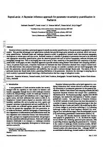
Fig. 1. (A) Generative model of the microstructure at the population level. Circles are random variables and shaded circles have observations. Indices relate to fascicles and superscripts to subject (omitted in the text for clarity). The left box is repeated for the N fascicles in the voxel and the whole is repeated for all V voxels. (B) Instances of logistic-normal distribution over the simplex and Watson distribution over the sphere.

inferring a joint posterior probability over the model parameters. The posterior probability can then be interrogated to answer research questions [1]. Defining a generative model of the microstructure at the population level, however, is challenging due to the geometry of the space of parameters. This paper tackles this challenge and presents a novel Bayesian inference framework for population studies the brain microstructure. Section 2 presents our assumptions. Section 3 and 4 describe our model and its inference. Section 5 shows experimental results.

2

Parameterization and Assumptions

Multi-fascicle models represent the signal from each compartment in each voxel as a separate Gaussian encoded by a tensor D i , weighed by fi [6]: S(b, g) = S0

N X

fi e−bg

T

Di g

, where b is the b-value and g is the gradient.

i=1

One tensor is isotropic [4,5,6] and the two smallest eigenvalues of each tensor are equated and represent the radial diffusivity [4]. The biophysical properties of this model are: the vector di = (dk,i , d⊥,i ) of axial and radial diffusivities and the principal direction ei of Fascicle i, and the vector of fractions f. These variables have observations dji , eji and f j for Subject j. Inter-subject variability in these properties (encoded in the likelihood) is assumed much larger than DWI noise. An extra level in the hierarchical model could otherwise link parameters to DWI [9]. Fascicles are assumed independent from one another. By symmetry, directions are independent from diffusivities and fractions. Signal fractions mostly relate to partial voluming and are thus independent from fascicle properties. Diseases may affect several properties of the microstructure, so that these assumptions are only valid conditional on the diagnoses. In summary, we have: di =(d ˆ k,i , d⊥,i ), di ⊥ ⊥ dj6=i ,

ei ⊥⊥ ej6=i ,

ei ⊥⊥ di ,

ei ⊥⊥ f,

and f ⊥⊥ di .

3

Model

˜ principal Fig. 1 shows our hierarchical model for the latent diffusivities (δ, δ), directions (εi , ε˜i ) and signal fractions (ϕ, ϕ) ˜ for the control and patient (tilded) groups respectively. Owing to the biophysical parameterization of the model, the posterior for these variables is of the form (conditioning on diagnoses is implicit): ˜ ε, ε˜, ϕ, ϕ|f p(δ, δ, ˜ , D) = p(ϕ, ϕ|f ˜ )

N Y i=1

p(δ i , δ˜i |di )p(εi , ε˜i |ei ).

A fully Bayesian hierarchical model is obtained by representing unknowns as random variables and assigning priors over their value [1]. We assign uniform priors for bounded variables, and log-normal priors for unbounded positive-definite variables. The log-normal prior only requires a vague idea about the order of magnitude of the variable, encoded as its mean. Its standard deviation is set to 5 to allow for mistakes in our estimate of the order of magnitude. Modeling diffusivities. Diffusivities are in R+ ×R+ . We represent distributions over their logarithm to assign zero probability to negative values [8]. The inter-subject variability within a group is represented as a normal law: ˜i ˜ δ i , Σdi ∼ N (log δ˜i , Σdi ). log di δ i , Σdi ∼ N (log δ i , Σdi ) and log d A prior over (δ i , δ˜i ) is best expressed conditionally: p(δ i , δ˜i ) = p(δ˜i |δ i )p(δ i ). The order of magnitude of diffusivities is around 10−4 , 10−3 mm2 /s, so δ i ∼ log N (−3.5, 5). Given δ i and without data from patients, our best guess for δ˜i is δ i , which we encode as δ˜i δ i , αi ∼ log N (log δ˜i , αi2 I 2 ) for an unknown variance αi2 . We assign a log-normal hyperprior to αi with zero mean, to express that δ˜i and δ i likely have, a priori, a similar order of magnitude. Regarding Σdi , the correlation between the axial and radial diffusivities is unknown a priori whereas we have a vague idea of the order of magnitude of the standard deviation of each diffusivity. This prior information is effectively encoded by factorizing Σdi = diag(σ di )Cdi diag(σ di ) [1], where σ di is the vector of standard deviations and Cdi is a 2 × 2 correlation matrix. We assign a log-normal prior to σ di with zero mean to express that diffusivities likely have the same order of magnitude, and a uniform prior on [−1, 1] for the correlation coefficient in Cdi . Modeling directions. Directions are dipoles on the sphere. We model their likelihood as a Watson distribution [7], with unknown concentrations κi , κ ˜i : p(ei |εi , κi ) = A(κi ) exp (κi (εi  ei )) , p(˜ ei |˜ εi , κ ˜ i ) = A(˜ κi ) exp (˜ κi (˜ εi  ˜ ei )) .

We express the priors over latent group variables conditionally: p(εi , ε˜i ) = p(˜ εi |εi )p(εi ). The prior p(εi ) is uniform over the sphere and, conditionally on εi , we model our prior knowledge about ε˜i as another Watson distribution with mean εi and unknown concentration βi . At concentrations of 10−5 , the Watson is essentially uniform and at 105 , it is extremely peaky. We therefore assign iid log-normal hyperpriors to all concentration parameters βi , κi , κ ˜ i ∼ log N (0, 5).

P Modeling fractions. Fractions belong to an N -simplex: {f , fi ≥ 0, i fi = 1}. The conventional Dirichlet density, with a single parameter for all variances and covariances, is too limited to represent their likelihood. Instead, we apply a change of variables to map f to an (N − 1)-vector of unconstrained variables y: ! fi y=F ˆ (f) : yi = Fi (f) = logit + log (N − i) . Pi−1 1 − i0 =1 fi0 The logit maps its argument from (0, 1) to (−∞, +∞). The second term is added so that y = 0 ⇔ fi = 1/N, ∀i. We model the likelihood of y as a multivariate normal distribution with mean F (ϕ) for controls, F (ϕ) ˜ for patients and unknown covariance Σf . This leads to a normal logistic distribution (Fig. 1B) whose expression is derived from the Gaussian density and the Jacobian of F : QN 1   1 i=1 fi T −1 exp − (F (f) − F (ϕ)) Σf (F (f) − F (ϕ)) . p(f|ϕ, Σf ) = 1/2 2 |2πΣf | A non-informative prior on ϕ is obtained by a normal with large variance: F (ϕ)∼N (0, 1000I N −1 ). F (ϕ)|F ˜ (ϕ) is assigned a multivariate normal prior with mean F (ϕ) and covariance γI N −1 with unknown γ. As for αi and βi , γ is assigned a log-normal hyperprior with zero mean. The unknown covariance is decomposed as Σf =diag(σf )Cf diag(σf ). The correlation Cf is an (N −1)×(N −1) matrix to which we assign a LKJ(η=1) prior which is uniform over all correlation matrices [1]. As before, σf is assigned a log-normal prior with zero mean.

4

Inference

The model needs to be estimated in each voxel. Efficient estimation of its posterior is therefore critical to its use in practice. The posterior has no closed-form expression due to interactions between variables and the introduction of nonconjugate priors. Variational Bayes approximations, often used in this case, may introduce biases that would jeopardize the reliability of group differences [2]. We therefore use Markov Chain Monte Carlo (MCMC) sampling. Because our logposterior is differentiable, we exploit Hamiltonian Monte Carlo (HMC) sampling which converges much faster (in O(D5/4 ) for D dimensions) than conventional Gibbs and Metropolis sampling (O(D2 )) [2]. Specifically, we use the No-U-Turn Sampler (NUTS) which automatically optimizes the parameters of the HMC sampling [2]. We draw four Markov chains of 2000 samples and discard the first 1000 burn-in samples. Convergence is monitored by the scale reduction factor ˆ [1]. From samples of the joint posterior over the model parameters θ (all R variables in Fig. 1), marginal posteriors of any statistics of interest T(θ) are simply obtained by computing their values from the posterior samples. Importantly, because the joint posterior is not altered by the computation of T(θ), many statistics can be simultaneously analyzed without the need to correct for multiple comparisons as in NHST. False discoveries are mitigated by the shrinkage towards the prior. For the validation, we focus on the posterior probabilities

Number of subjects 20 30 40 1

1

1

0

1

1

0

1

0

1

0.6

1

0

0

0

1

0

1

0

1

1

0

1

0.6

1

0

1

0

0.6

1

1

1

0

0.6

1

0

1

0.6

0

1

1

0.6 1

0.6 1

0.6 1

0.6 1

0.6

0.6

0.6

0.6

= 40 0.6

3

0

= 20 1

2

50

= 10

Our approach

Rician noise level

1

1

10

1

(D) ROC

0.6

(C) One patient (σ=40)

1

(B) Patient template

NHST

(A) Control template

1

(E) Ground truth

(F) NHST (J=10)

(G) NHST (J=50)

(H) Our approach (J=10) (I) Our approach (J=50)

0

Fig. 2. (A) Template for the control population (fractions encoded as RGB). (B) Template for the patient population with three overlapping affected areas (see text). (C) A simulated patient with noise at level σ = 40. (D) ROC analysis demonstrates that our approach outperforms NHST for all noise levels and all number of subjects. (E) Ground truth difference in radial diffusivity. (F-G) NHST provides evidence for an alteration in Area 1 but fails to provide evidence that no alteration is present elsewhere. Color encodes 1 − p-value. (H-I) Bayesian posterior maps provide both evidence that fascicles in Area 1 are altered (high posterior) and that tensors elsewhere are unaltered (low posterior). This evidence increases as the number of subjects increases.

that the differences in latent group variables fall outside a region of practical equivalence (ROPE):  

P |δ.,i − δ˜.,i | > d Data , P |ϕi − ϕ˜i | > f Data , P |acos(εi  ε˜i )| > e Data . The bounds of ROPE vary with the empirical context. In our experiments, we set d =10−6 mm2 /s, f =0.01, e =1◦ . Posterior values close to 1 are strong evidence for the presence of a microstructure abnormality, akin to small p-values in NHST. Posterior values close to zero are strong evidence that the difference between the groups is within the ROPE. This property of the posterior has no equivalent in NHST and has, as will be seen, far-reaching consequences in population studies.

5

Experiments and Results

Implementation. HMC sampling was implemented in Stan 2.2 (mc-stan.org), ˆ = 1). took an average 0.03 sec per chain and always reached full convergence (R Data. Directly simulating multi-fascicle models is biased because the impact of the noise on model parameters is unclear. We therefore simulated the process of estimating models from noisy DWI. We created a control and a patient template with various crossing angles (Fig. 2A-B). The patient template has overlapping areas of microstructural differences: Area 1 has radial diffusivity of oblique fascicles inflated by 10%, Area 2 has in-plane orientation alterations of 10◦ and Area

(A)

NHST

(C) Our approach multivariate analysis

(B)

Our approach

NHST

RMSE (lower is better)

Our approach

Direction Direction

(D)

Bayesian Fascicle-Based Spatial Statistics

1.6x10-3mm2/s

Radial Radial MD MD Fraction Fraction

0

0.35

C P k , k

Experiment

Axial Axial

0 1

1

1

0

0

0 6x10-4mm2/s

Patients Controls Position along the fascicle

Direction Direction

Independent replication

Axial Axial Radial Radial

MD MD Fraction Fraction 0.4

C P ?, ?

Cohen’s Kappa (higher is better)

0

Patients Controls Position along the fascicle

0.6

Fig. 3. (A) RMSE and Cohen’s κ coefficient both indicate that inference results from the Bayesian approach are more reproducible than those obtained with NHST. (B) The improved reproducibility for the axial diffusivity is explained by the presence of many voxels with low values of the posterior (blue voxels) for which NHST results in uniformly distributed p-values. (C) Our framework can be applied to more complex analyses such as the coupled increase in fraction of isotropic diffusion and radial diffusivity. The resulting posterior map can be interpreted exactly as the others. (D) Augmenting the model with spatial priors enables the analysis of fascicle-wise properties, such as the diffusivity profile along the arcuate fasciculus.

3 has increased fraction of isotropic diffusion by 0.1. For each simulated subject, 90 DWI on 3 shells at b=1,2,3000, were corrupted by Rician noise with scale parameters σ = 10, 20, 40. Multi-fascicle models were then estimated as in [6] (Fig. 2C). For each σ, groups of K patients and K controls were generated for K = 10, 20, 30, 40, 50. The process was repeated 10 times for each pair (σ, K) leading to 150 synthetic populations. In-vivo DWI (1.7×1.7×2mm3 , Siemens 3T Trio, 32-channel head coil) were acquired using the CUSP-45 sequence [6] with b-values up to 3000 in 36 patients with Tuberous Sclerosis Complex (TSC), a condition with high prevalence of autism, and 36 age-matched controls. Twofascicle models with one isotropic compartment were estimated. Preprocessing. All multi-fascicle models were non-linearly registered to an atlas as in [8]. At each voxel, the tensors of all J controls and K patients were grouped in N clusters using the iterative scheme of [8], where N is the number of fascicles in the atlas. Due to model selection, the number of observations (Ji +Ki ) varies between fascicles. The presence or absence of a fascicle may itself be an interesting group contrast and is reflected in the vector of fractions f that may contain null values (replaced by an epsilon machine to avoid singularity). Validation on synthetic phantoms. Population studies were conducted with all 150 simulated populations and for five properties: the radial, axial and mean diffusivities, the orientation of fascicles and the fractions of isotropic diffusion. NHST for log-diffusivities and logit-fractions were performed by independent ttests as in [8] and NHST for directions used Schwartzman’s test for diffusion

tensors [7]. For all properties, true positive rates and true negative rates were computed at different thresholds leading to ROC curves (Fig. 2D). Consistently for all noise levels and all number of subjects, our Bayesian approach outperforms NHST. This is also the case independently for each property that presents a group contrast. The improvement of our Bayesian approach over NHST is akin to tripling the number of subjects. This can be attributed to two features of the Bayesian framework. First, the introduction of ROPE avoids the detection of false positives with negligible yet statistically significant magnitude. Second, low values of the Bayesian posteriors is evidence for the absence of a group difference whereas high p-values occur randomly (uniformly) if the null hypothesis is true. This situation is illustrated in Fig. 2E-I for the radial diffusivity. Bayesian posteriors outside of Area 1 takes on small values (Fig. 2H-I) whereas p-values are uniformly distributed in those voxels. Validation on in-vivo data. In-vivo data were used to assess the reproducibility of results. Patient and control groups were each split in two subgroups, leading to two cohorts each with 18 controls and 18 patients. Population studies for directions, isotropic fraction, radial, axial and mean diffusivities were conducted in each cohort. For each property, the resulting two p-value maps were compared to one another in terms of root mean squared error (RMSE) and so were the two posterior maps. For all five variables of interests, the RMSE was significantly smaller between posterior maps (mean RMSE: 0.23) than between p-value maps (mean RMSE: 0.32; two-sample t-test: p < 0.0005) with a mean improvement of 27.5% (Fig. 3A). The largest improvement was observed for the axial diffusivity (reduction of 35%). RMSE directly compares the statistical maps regardless of the decision made from these maps (after thresholding). We therefore also assess reproducibility of inference results based on Cohen’s κ coefficient of agreement a −Pe where Pa after thresholding p-values at 0.05 and posteriors at 0.95: κ = P1−P e is the observed agreement probability and Pe is the probability of agreeing by chance. κ was larger with the Bayesian approach for all properties except for the directions (Fig. 3A). The improvement was larger for axial diffusivity (+6.5%). The higher improvement in reproducibility observed for the study of axial diffusivity both in terms of RMSE and κ is elucidated by Fig. 3(B). Strong evidence for the absence of any substantive difference in axial diffusivity can be inferred and reproduced with the Bayesian approach (blue areas in Fig. 3B). In these regions, the p-value is uniformly distributed leading to poor RMSE and κ. Prospectives. So far, we focused on simple statistics to fairly compare our approach to NHST. But more complex statistics may too be of interest. For instance, the presence of myelin injury with neuroinflammation may result in a coupled increase in fraction of isotropic diffusion due to cell swelling and in radial diffusivity due to demyelination. This association remains hypothetical, but our capability to detect it may increase specificity of microstructure imaging. Detection of these complex responses is not easily framed as an NHST, but is readily computable with our Bayesian approach: p(ϕ˜iso > ϕiso , δ˜⊥,i > δ⊥,i Data), depicted in Fig. 3C. Our Bayesian framework also enables incorporation of prior

information, such as spatial priors to increase coherence of the posterior. To illustrate this possibility, we augment our model with a Gaussian Markov random field prior over latent diffusivities in adjacent voxels along a fascicle of interest: the median tract of the left arcuate fasciculus (AF). The results are joint posteriors of all diffusivities along the tract, leading to fascicle-wise (rather than voxel-wise) analysis. The profiles in Fig. 3D are maximum a posteriori (lines) and 95% posterior intervals (shades). They indicate that TSC patients have substantially higher radial but unaltered axial diffusivities along the AF.

6

Conclusion

This paper introduced a Bayesian framework to conduct population studies of the brain microstructure. A key property of this framework is its ability to build evidence for the absence of alterations alongside the detection of abnormalities. This key property makes it less prone to false discoveries than NHST and improves reproducibility of findings. By estimating the full posterior distribution over latent variables, our Bayesian framework therefore enables richer and more reliable analyses of the brain microstructure and its alterations in diseases. Acknowledgments This work was supported in part by F.R.S.-FNRS, WBI, NIH grants R01 NS079788, R01 LM010033, R01 EB013248, P30 HD018655, and by a research grant from the Boston Children’s Hospital Translational Research Program.

References 1. Gelman, A., Carlin, J.B., Stern, H.S., Dunson, D.B., Vehtari, A., Rubin, D.B.: Bayesian data analysis. CRC press (2013) 2. Hoffman, M.D., Gelman, A.: The no-U-turn sampler: Adaptively setting path lengths in Hamiltonian Monte Carlo. Journal of Machine Learning Research (2013) 3. Nuzzo, R.: Scientific method: statistical errors. Nature 506(7487), 150–152 (2014) 4. Panagiotaki, E., Schneider, T., Siow, B., Hall, M.G., Lythgoe, M.F., Alexander, D.C.: Compartment models of the diffusion MR signal in brain white matter: a taxonomy and comparison. Neuroimage 59(3), 2241–2254 (2012) 5. Pasternak, O., Westin, C.F., Bouix, S., et al.: Excessive extracellular volume reveals a neurodegenerative pattern in schizophrenia onset. The Journal of Neuroscience 32(48), 17365–17372 (2012) 6. Scherrer, B., Warfield, S.K.: Parametric representation of multiple white matter fascicles from cube and sphere diffusion MRI. PLoS one 7(11), e48232 (2012) 7. Schwartzman, A., Dougherty, R., Taylor, J.: Cross-subject comparison of principal diffusion direction maps. Magnetic Resonance in Medicine 53(6), 1423–1431 (2005) 8. Taquet, M., Scherrer, B., Commowick, O., Peters, J.M., Sahin, M., Macq, B., Warfield, S.K.: A mathematical framework for the registration and analysis of multifascicle models for population studies of the brain microstructure. Medical Imaging, IEEE Transactions on 33(2), 504–517 (2014) 9. Taquet, M., Scherrer, B., Boumal, N., Macq, B., Warfield, S.K.: Estimation of a multi-fascicle model from single b-value data with a population-informed prior. In: Mori, K., Sakuma, I., Sato, Y., Barillot, C., Navab, N. (eds.) Medical Image Computing and Computer-Assisted Intervention, LNCS, vol. 8149, pp. 695–702 (2013)