Apr 7, 2006 - as FELICS algorithm [12], those algorithms have no good compression performance for Bayer image data. The com- parison results between ...
Hindawi Publishing Corporation EURASIP Journal on Advances in Signal Processing Volume 2007, Article ID 82160, 13 pages doi:10.1155/2007/82160
Research Article A Near-Lossless Image Compression Algorithm Suitable for Hardware Design in Wireless Endoscopy System Xiang Xie, GuoLin Li, and ZhiHua Wang Department of Electronic Engineering, Tsinghua University, Beijing 100084, China Received 12 September 2005; Revised 28 February 2006; Accepted 7 April 2006 Recommended by Liang-Gee Chen In order to decrease the communication bandwidth and save the transmitting power in the wireless endoscopy capsule, this paper presents a new near-lossless image compression algorithm based on the Bayer format image suitable for hardware design. This algorithm can provide low average compression rate (2.12 bits/pixel) with high image quality (larger than 53.11 dB) for endoscopic images. Especially, it has low complexity hardware overhead (only two line buffers) and supports real-time compressing. In addition, the algorithm can provide lossless compression for the region of interest (ROI) and high-quality compression for other regions. The ROI can be selected arbitrarily by varying ROI parameters. In addition, the VLSI architecture of this compression algorithm is also given out. Its hardware design has been implemented in 0.18 µm CMOS process. Copyright © 2007 Hindawi Publishing Corporation. All rights reserved.
1.
INTRODUCTION
Compared to the conventional endoscopy system, the wireless capsule endoscopy allows us to directly study the entire small intestine and does not require any sedation, anesthesia, or insufflation of the bowel. There is the only clinic device made by Israel in the world [1]. However, it can only work for less than eight hours (generally, it costs capsule about 10–48 h, typically 24 h, on moving from mouth to evacuation [1]) and the image frame rate is slow (2 frames/second), which results in the fact that there is not enough time for the capsule to check the large intestine, and some regions interesting to the doctors are often missed. By analyzing power consumption in capsule, it can be known that the power of transmitting image data occupies about 80% of the total power in capsule. In the digital wireless endoscopy capsule system designed by us, the power is supplied by two batteries and a CMOS image sensor is used [2]. In order to reduce the communication bandwidth and the transmitting power in the capsule, the image compression has to be applied. Although the CMOS sensors will bring some noises to the captured images, it does not affect the doctor’s diagnosis. Once the lossy compression is used, some information contained in the original images will be lost, which results in the error diagnosis. So a new low-complexity and high-quality image compression for digital image sensor with Bayer color filter arrays needs to be used [2]. Figure 1 shows the simplified
block diagram of our wireless endoscopy capsule system. The output image data from a CMOS image sensor is compressed first and then coded by channel coding module. Finally, the data are transmitted by a wireless transceiver to the outside of the body. The transmitted data will be received and decompressed for subsequent diagnosis. The control unit in capsule controls the compression module according to the received commands from the external remote control. Some compression algorithms for Bayer format image data have been reported to get higher-compression performance [2–7]. However, all those algorithms are proposed for lossy compression and are not suitable for the medical image compression in the wireless endoscopy system. Toi and Ohita applied the subband coding technique in the compression first scheme [4]. The technique cannot be used for near-lossless or lossless image compression because the diamond filter used cannot be reconstructed perfectly. Lee and Ortega [5] gave a reversible image transformation. The RGB is transformed to YCbCr firstly. Then Y data array is rotated into a rhombus. Finally the rotated Y data, original Cb, and Cr data are compressed by JPEG separately. However, since the rotated Y data is not rectangular, the standard encoder, such as JPEG-LS, JPEG, and JPEG2000, cannot be applied directly. Recently, Koh et al. [6] presented two new methods: “structure conversion” method and “structure separation” method. Essentially, the key difference between the two methods is that two different low-pass filters are applied. The
2
EURASIP Journal on Advances in Signal Processing
COMS image sensor
Bayer data
Image compression
Channel coding
Wireless transceiver
Channel decoding
Control unit
Figure 1: Block diagram of system architecture inside wireless endoscopic capsule.
G
B
G
B
R
G
R
G
G
B
G
B
R
G
R
G
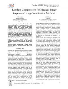
Figure 2: Bayer pattern color filter array (CFA).
computational complexity of structure conversion method is lower than that of structure separation method. The structure separation method is unsuitable for near-lossless or lossless image compression because of the nonreversible diamond filter. Although [8] presents a new lossless compression based on wavelet transformation, its computation complexity is so high for wireless endoscopy application. This paper presents a new near-lossless image compression algorithm for the wireless endoscopy system. It has low complexity hardware implementation and supports real-time compressing. In this paper, PSNR larger than 46.37 dB and no more than 2 intensity levels error for a pixel is defined as near-lossless. This strict definition assures high image quality, which is safe for patient diagnosis. The color filter arrays (CFAs) data discussed in this paper is the most popular Bayer pattern [9] as illustrated in Figure 2. 2.
PROPOSED NEAR-LOSSLES COMPRESSION ALGORITHM
2.1. Algorithm structure A simple structure for the proposed near-lossless compression algorithm is illustrated in Figure 3(a). In this algorithm, before image compression, there is a data preprocessing part which includes image format transformation and a low-pass filter. First, the Bayer pattern CFA data is transformed into a format suitable for image compression as well as for hardware design. The data is then low-pass filtered directly in RGB space. JPEG-LS [10] is used here for low complexity of hardware implementation and high efficient compression performance. Some other lossless compression coders such as CALIC [11] have better compression performance, but they have much more computational complexity than JPEGLS, which is not suitable for the low-power design inside
the wireless endoscopic capsule. Although there are some other lower complexity lossless compression algorithms such as FELICS algorithm [12], those algorithms have no good compression performance for Bayer image data. The comparison results between FELICS and JPEG-LS for Bayer image data will be given in Section 4. The introduction of the low-pass filters leads to a small loss of high frequency, but a low-compression rate with high fidelity can be obtained. The reconstructed image quality can be adjusted by changing the quality control factor. Moreover, the specified ROI can be coded without loss by adjusting the ROI parameters. The quality control factor and ROI parameters are used as the input parameters of the low-pass filter. The corresponding decompression algorithm is shown in Figure 3(b). It is a simple reverse procedure of the compression. 2.2.
Analysis of the algorithm structure
There are two compression methods for the Bayer format image data. The first method is to compress Bayer data directly, and the other is to compress G, B, and R components, respectively. The proposed algorithm illustrated in Figure 3 belongs to the first method. In general, in the second method, G, B, and R components of Bayer data are preprocessed and then compressed, respectively, as in [2–8]. This method structure can be shown in Figure 4. Two major structures of this method are illustrated in this figure. One is the “serial structure” in which three components are compressed one by one, and the other is “parallel structure” in which three components are compressed parallel. Only from the viewpoint of the compression performance, the second method is better than the first method because this method makes full use of the correlation between neighbor pixels in the same color plane. However, the second method needs much more hardware overhead than the first method. The reason is illustrated in the following. In a CMOS image sensor, there are some different readout modes such as progressive scan and interlaced scan. Assume the size of the raw Bayer data is 4 ∗ 4, take the progressive scan as an example, the raw Bayer image data are read out as shown in Figure 5. In serial structure of Figure 4(a), when G component is being compressed, the other two components have to be saved in a buffer. Three components have to be compressed one by one in turn, which results in the fact that the compression cannot be implemented in pipeline hardware structure. Compared to the first method, the “serial
Xiang Xie et al.
3 Preprocessing Quality control factor ROI parameter Image format Low-pass transformation filter
Raw Bayer data
JPEG-LS encoding
Compressed data
(a)
Quality control factor ROI parameter
Restored Bayer data
Image format transformation
JPEG-LS decoding
Reconstruction filter
Compressed data
(b)
Figure 3: Block diagrams: (a) the proposed near-lossless compression algorithm and (b) the corresponding decompression algorithm.
Switch Raw Bayer data
G
B&R
Preprocessing
Lossless or lossy encoding
Preprocessing
RAM (half image size)
Compressed data
(a) Serial compression structure
G
Raw Bayer data
Preprocessing
Lossless & lossy encoding (1)
Preprocessing
Lossless & lossy encoding (2)
R Preprocessing
Lossless & lossy encoding (3)
B
Compressed data
(b) Parallel compression structure
Figure 4: G, B, and R are compressed, respectively.
B
G
B
G
G
R
G
R
B
G
B
G
G
R
G
R
Figure 5: Progressive scan sequence of a CMOS image sensor.
structure” needs more additional buffer with half image size to store R and B components, and moreover, it is not suitable
for real-time compressing. As the captured image size becomes larger, the buffer size also becomes larger. In our endoscopy system, the captured image size is 640 ∗ 480 ∗ 8 bits and the designed endoscopic capsule size is smaller than 9 ∗ 20 mm. Even if we use the 0.18 µm CMOS process to design the chip inside the capsule, the ram buffer with 640 ∗ 480 ∗ 8 ∗ 0.5 = 1 228 800 bits size is too large to be installed in that miniature capsule. The “serial structure” illustrated in Figure 4(a) limits the captured image size. Moreover, the fact that three components have to be compressed one by one limits image processing speed and makes it very difficult to realize real-time endoscopic image monitoring. In the “parallel structure” illustrated in Figure 4(b), three same encoding modules have to be used. Compared to the first method illustrated in Figure 3, this method will result in triple logical
4
EURASIP Journal on Advances in Signal Processing
hardware overhead and about triple power consumption. So, the first method is used in our system. 2.3. Algorithm description There are more high-frequency components in the horizontal and vertical directions of the Bayer CFA data than that in the full-color image data, which is disadvantageous to image compression. In order to avoid this problem, first, the data format is transformed as illustrated in Figure 6. All the quincunx G components are moved to the left side to decrease the high frequency in raw Bayer data. Although the B and R components are interlaced after transformation, the compression performance is affected very little. Note that the buffer expenditure of the transformation is only two lines at most. Here, one line length equals image width. Then the raw Bayer data should be smoothed to further decrease the highfrequency components as follows. The pixels of the first row are not filtered while other pixels are filtered row by row. The array of the low-pass filter is described in (1), but its filtering operation is different from the regular operation. The low-pass filter scans from the second row until the last row is reached, as illustrated in Figure 7. The scan sequence is the same as that of readout mode of the image sensor. The virtual pixel(n) of the left boundary is equal to its nearest right pixel in the first column, and the virtual pixel of the right boundary is equal to its nearest left pixel in the last column. Those virtual pixels are used to compute left and right boundary points in the filtering operation. The circled number in this figure represents the scan sequence of the filter operation. Note that the filtered pixels are used for the filtering operation of the following next neighboring rows. For example, in Figure 7(b), the filtered pixels of the second row are used for the filtering operation of the third row. After the filtering operation, Bayer data arrays will become smoother. So the compression rate can be improved. The proposed low-pass filter has three key merits. The first is its simplicity. For example, compared with the filter used in [4, 8], the proposed filter has much lower complexity. The second is its low-pass character. The last merit is its perfect reconstruction: ⎡
⎤
⎢1 1 1⎥ ⎥ 1⎢ ⎢ ⎥ ⎥. Hbr = ⎢ 0 1 0 ⎥ 4⎢ ⎣ ⎦
(1)
0 0 0 Moreover, the perfect and simple reconstruction filter can be obtained for high image quality. The reconstruction � matrix is Hbr and the reconstruction filtering operation can be illustrated in Figure 8: ⎤
⎡ � Hbr
⎢−1 −1 −1⎥ ⎥ ⎢ ⎥ ⎢ = ⎢ 0 4 0 ⎥. ⎥ ⎢ ⎦ ⎣
0
0
0
2.4.
Rounding operation
The coefficient in matrix (1), 1/4, makes the division operation or shift operation unavoidable in the filtering process. Its residual values are 0, 1, 2, or 3. To reduce the residual error, the rounding operation is applied. It is described simply in the following equation: �
(3)
Here, “�•�” is the integer-valued operator (�•� ≤ •), x and y are integers, and y is the rounded result. In this compression algorithm, (3) is expanded into a matrix equation as follows: Om×n =
1 � × Im×n ⊗ Hm×n + Em×n 4
m×n
.
(4)
In (4), � X �m×n represents the integer-valued operator of the m × n matrix X. The integer value of every element in the matrix � X �m×n is not larger than that of the element of corresponding position in the matrix X, that is, � X �m×n ≤ X. Om×n denotes the matrix of the filtered data, Im×n denotes the m × n matrix of original CFA data, H denotes the lowpass filter, and Em×n denotes an m × n matrix in which the values in the location of all filtered elements are ones. 2.5.
Error analysis
In the proposed algorithm, the implementation precision is 8-bit. The error is generated only by the division operation in the low-pass filter. If there is no rounding operation, the absolute error between the original CFA data and the filtered data is expressed in the following equation: � �
e1 = � �x − 4 ×
� � 1 ×x � �. 4
(5)
Here, x is an integer and e1 is the absolute error. From this equation, e1 ≤ 3 can be deduced, that is, the maximum absolute error is three. Table 1 shows the residue value distribution in seven-color images with Bayer CFA pattern and size 512 × 512. These images are generated from seven standard test images. Because the size of each image is 512 × 512, the summation of every column in Table 1 is 262 144. From Table 1, statistical analysis yields the approximate probability distribution of e1 : 1 p(0) = p(1) = p(2) = p(3) = . 4
(6)
When the rounding operation is used, the absolute error,e2 , between the original data and filtered data can be described as follows: � �
(2)
1 (x + 1) . y= 4
e2 = � �x − 4 ×
� � 1 × (x + 1) � �. 4
(7)
From (7), e2 ≤ 2 is obtained. After the rounding operation, the maximum absolution error is reduced to two. The error
Xiang Xie et al.
5 Image format transformation G11 B12 G13 B14 G15 B16 G17 B18
G11 G13 G15 G17 B12 B14 B16 B18
R21 G22 R23 G24 R25 G26 R27 G28
G22 G24 G26 G28 R21 R23 R25 R27
G31 B32 G33 B34 G35 B36 G37 B38
G31 G33 G35 G37 B32 B34 B36 B38
R41 G42 R43 G44 R45 G46 R47 G48
G42 G44 G46 G48 R41 R43 R45 R47
G51 B52 G53 B54 G55 B56 G57 B58
G51 G53 G55 G57 B52 B54 B56 B58
R61 G62 R63 G64 R65 G66 R67 G68
G62 G64 G66 G68 R61 R63 R65 R67
G71 B72 G73 B74 G75 B76 G77 B78
G71 G73 G75 G77 B72 B74 B76 B78
R81 G82 R83 G84 R85 G86 R87 G88
G82 G84 G86 G88 R81 R83 R85 R87
(a) Bayer pattern CFA data
(b) Transformed pattern data
Figure 6: Image transformation operation.
1
2
3
4
8
5
6
7
8
12
9
10
11
12
1
2
3
4
5
6
7
9
10
11
1
(a)
4
...
5
1
2
3
4
5
6
7
8
9
10
11
12
(b)
8
(c)
Figure 7: Filtering operation.
distribution with rounding operation is shown in Table 2. From this table, the approximate probability distribution of e2 , p(e2 ), can be obtained as follows: 1 p(0) = p(2) = , 4
1 p(1) = . 2
(8)
In fact, after filtering a large amount of images, the same statistical probability distribution of the errors can be gotten. The error value is focused on one and zero after rounding operation. In this paper, we define PSNR in the near-lossless compression, the measure of image quality, as follows:
⎛
PSNR = 10 log10 ⎝
(1/H × W)
I1 and I2 are original and reconstructed images with height H and width W, respectively, and are expressed in integer values between 0 and 255, and x and y are locations of pixels.
�
PSNR = 10 log10
⎞
2552
�W �H � x=1
y =1
I1 (x, y) − I2 (x, y)
2 ⎠ ;
According to the error distribution in (8) and the defined PSNR equation (9), the statistic image quality after filtering is
2552 � 1/(H × W) • p(1) • (H × W) • 12 + p(2) • (H × W) • 22 �
(9)
� = 46.37.
(10)
6
EURASIP Journal on Advances in Signal Processing
1
2
3
4
1
2
3
4
5
6
7
8
5
6
7
8
9
10
11
12
9
10
11
12
(a)
...
5
1
2
3
4
5
6
7
8
9
10
11
12
(b)
8
(c)
Figure 8: The reconstruction filtering operation.
Table 1: Residue distributions of Bayer data without rounding operation. These Bayer CFA data are generated from seven standard test color images with size 512 × 512 e1
Airplane
Baboon
House
Lake
Lena
Peppers
Splash
0
65586
65855
65233
66065
65747
66012
66119
1
65712
65250
66234
65317
65106
65130
65245
2
65365
65520
65942
65307
65526
65867
65712
3
65481
65519
64735
65455
65765
65135
65068
2.6. Adjustable image quality and compression rate By decreasing the number of CFA data to be filtered, the image quality, PSNR, can be increased. In the proposed algo-
�
PSNR = 10 log10
rithm, the percent of the data to be filtered in CFA raw data is used as an input parameter, that is, the quality control factor in Figure 4. The PSNR can be described in the following equation:
2552 � � (1/H × W) • p(1) • (H × W × q) • 12 + p(2) • (H × W × q) • 22
Here, “q” is the quality control factor and 0 ≤ q ≤ 1. When q = 0, there is no low-pass filter in the algorithm. Equation (10) shows the minimum PSNR when q = 1. From (11), any PSNR larger than 46.37 dB can be gotten by changing the input parameter q. In theory, the worst case is that the error of every filtered pixel is 2, the PSNR is larger than 42.11 dB. In the practical natural images captured by the image sensor, the neighbor pixels have very strong correlation, so the PSNR in statistics is larger than 46.37, which is shown as illustrated in (11). A simple way that the selection of rows to be filtered instead of the selection of pixels is used. Those selected rows are distributed equally in CFA raw data. For example, in Figure 9(a), assuming that the size of CFA data is eight by eight and q = 0.5, the pixels in odd rows except for the first row, that is, pixels in the 3rd, 5th, and 7th rows, are filtered and other original pixels are compressed directly
� = 46.37 − 10 log10 q.
(11)
by JPEG-LS, and the PSNR of the reconstructed CFA data is 46.37 − 10 log10 0.5 = 49.37. Figure 9(b) shows the selection of the rows to be filtered when q = 0.25. The flow of the proposed near-lossless and lossless compression algorithm can be described in Figure 10. 2.7.
Lossless compression of ROI
In the proposed algorithm, the processing of ROI is very simple. The lossless compression of ROI is realized by this way that the pixels in ROI are not filtered by the low-pass filters according to the ROI parameters which contain the information of location and shape of ROI. For example, in Figure 11, assuming that the size of CFA data is eight by eight and the ROI is in a 2 ∗ 2 dashed rectangle, so the pixels in the dashed rectangle, G44, R45, B54, and G55, are not filtered.
Xiang Xie et al.
7
Table 2: Residue distributions of Bayer data with rounding operation. These Bayer CFA data are generated from seven standard test color images with size 512 × 512 Baboon
House
Lake
Lena
Peppers
Splash
0
65586
65855
65233
66065
65747
66012
66119
1
131193
130769
130969
130772
130871
130265
130313
2
65365
65520
65942
65307
65526
65867
65712
G11 B12 G13 B14 G15 B16 G17 B18
G11 B12 G13 B14 G15 B16 G17 B18
R21 G22 R23 G24 R25 G26 R27 G28
R21 G22 R23 G24 R25 G26 R27 G28
G31 B32 G33 B34 G35 B36 G37 B38
G31 B32 G33 B34 G35 B36 G37 B38
R41 G42 R43 G44 R45 G46 R47 G48
R41 G42 R43 G44 R45 G46 R47 G48
G51 B52 G53 B54 G55 B56 G57 B58
G51 B52 G53 B54 G55 B56 G57 B58
R61 G62 R63 G64 R65 G66 R67 G68
R61 G62 R63 G64 R65 G66 R67 G68
G71 B72 G73 B74 G75 B76 G77 B78
G71 B72 G73 B74 G75 B76 G77 B78
R81 G82 R83 G84 R85 G86 R87 G88
R81 G82 R83 G84 R85 G86 R87 G88
(a)
Filtered columns
Airplane
Filtered columns
e2
(b)
Figure 9: (a) When q=50%, (b) when q=25%, dashed lines are in the filtered columns.
Start Specify reconstructed image quality, PSNR
G11 B12 G13 B14 G15 B16 G17 B18 R21 G22 R23 G24 R25 G26 R27 G28 G31 B32 G33 B34 G35 B36 G37 B38
Get quality control factor q from equation (11) Select the rows to be filtered
R41 G42 R43 G44 R45 G46 R47 G48 G51 B52 G53 B54 G55 B56 G57 B58 R61 G62 R63 G64 R65 G66 R67 G68
Filtering and transformation operation
G71 B72 G73 B74 G75 B76 G77 B78
JPEG-LS
R81 G82 R83 G84 R85 G86 R87 G88
End
Figure 11: The ROI is in the 2 ∗ 2 dashed rectangle.
Figure 10: Flow of the proposed compression algorithm.
3.
VLSI ARCHITECTURE OF THE PROPOSED IMAGE COMPRESSION ALGORITHM
The VLSI architecture of the proposed image compression algorithm is shown in Figure 12. The Bayer CFA raw data from the image sensor is firstly preprocessed, which includes image format transformation and low-pass filtering operation. Then the filtered data is compressed by JPEG-LS. Finally, all
the compressed data is stored into the SRAM. The clock management is applied here to gate the clocks of those modules when they are in idle state. The compressed data is stored back to the SRAM so that the ARQ communication scheme can be used to assure the high-quality image communication [13]. In this architecture, SRAM is needed to store the compressed image data, and a dual port block memory is used as two line buffer for image format transformation.
8
EURASIP Journal on Advances in Signal Processing Buf for variable N Buf for variable C Buf for variable B Buf for variable A Regular mode
Clock management Preprocessing part
Two line buffer Bayer image data & synchronous signal Synchronization Filtering and format transformation
JPEG-LS Update variables SRAM Error prediction
Run mode
Run scanning & Run-length coding
Context determination
Communication with control unit
Golomb coding
G B R
Control unit of JPEG-LS
Figure 12: The VLSI architecture of the proposed image compression algorithm.
Control unit of JPEG-LS
Column Row counter counter Synchronous signal & Bayer image data
Synchronization
Bayer image data
8 Addr
Two line buffer
8 Data WE RD
8
8 Registers
JPEG-LS
Image format transformation
Mux 8
+
8
Figure 13: The VLSI architecture of the preprocessing part.
The detail VLSI architecture of the preprocessing part is proposed as illustrated in Figure 13. The synchronous signals from the COMS image sensor include vertical and horizontal synchronous outputs and pixel clock output. The synchronous signals are used to count the location of current pixel, that is, the column and row sequence number. According to the synchronous signal, the “control unit of JPEG-LS” controls which pixels should be filtered or not to realize lossless compression of ROI. The filtered or unfiltered data are then stored into SRAM. Only one eightbit adder is used here to implement filtering operation. Three eight-bit registers to store three values of the neighbor filtered pixels are needed. The hardware overhead of image format transformation and low-pass filter is very low. So, compared with the VLSI architecture of lossless image
compression, the proposed VLSI architecture needs only very small additional hardware expenditure for filtering module. The JPEG-LS includes the following modules. (a) “Control unit of JPEG-LS”: it implements the control of acquisition and storage of input raw Bayer data as well as the storage of the compressed data. It also controls how the clock management module managements the input clock of every module in JPEG-LS. (b) “Context decision”: this module will implement local gradient computation and quantization, quantized gradient merging, and mode selection. The decision result will be sent to “control unit of JPEG-LS.” (c) “Error prediction”: it implements predicting edge detection and correction from the bias as well as computing
Xiang Xie et al.
9 Table 3: Compression results for test image. CR means compression rate and � means infinity Image (512 × 512)
Airplane
Baboon
House
Lake
Lena
Peppers
Splash
PSNR (dB)
46.3798
46.3875
46.4073
46.3996
46.3898
46.5354
46.5320
CR (bits/pixel)
2.9845
4.8923
3.4873
4.0380
3.5192
3.5344
2.7825
Proposed algorithm without
PSNR(dB)
42.6656
42.7137
42.6672
42.7166
42.7032
42.8919
42.8609
rounding operation
CR(bits/pixel)
2.9845
4.8926
3.4870
4.0387
3.5193
3.5344
2.7826
PSNR (dB)
�
�
�
�
�
�
�
CR (bits/pixel)
4.7071
6.8816
5.2397
5.9125
5.3632
5.3141
4.5685
JPEG-LS near lossless
PSNR (dB)
45.1718
52.3809
45.1541
45.1337
45.1239
45.2419
45.2670
compression (1)
CR(bits/pixel)
3.0123
6.6935
3.9325
4.4080
4.8955
5.2372
4.8723
FELICS with the proposed
PSNR (dB)
46.4160
46.3914
46.4328
46.4011
46.4099
46.5528
46.5374
low-pass filter (q = 1)
CR(bits/pixel)
4.1916
5.6328
5.4711
5.5309
6.5132
7.0018
6.8462
G, B, and R respective compression
PSNR (dB)
46.4160
46.3914
46.4328
46.4011
46.4099
46.5528
46.5374
method
CR (bits/pixel)
2.9669
4.7781
3.4221
3.9098
3.3040
3.3564
2.5938
Proposed algorithm (q = 1)
JPEG-LS lossless compression
prediction error and modulo reduction of the prediction error in the regular mode. (d) “Update variables”: the variables A, B, C, and N are updated and saved in the corresponding buffers in this module. The required memory is 368 ∗ 16 (for variable A) + 368 ∗ 6 (for variable B) + 368 ∗ 8 (for variable C) + 368 ∗ 6 (for variable N) = 13 248 bits. So, the JPEG-LS hardware module consumes about 13.248 kbits memory to store those variables. (e) “Golomb coding” [14]: it encodes the mapped prediction residual by using the parameter k and performs the code word length limitation procedure. (f) “Run scanning and run length coding”: this module implements reading the Bayer image data and determining the run length as well as encoding the value of the length. 4.
EXPERIMENTAL RESULTS AND DISCUSSIONS
4.1. Compression performance comparison The performance of the presented near-lossless compression algorithm is evaluated by comparing it with the JPEGLS near-lossless compression with near-parameter. In this experiment, the CFA raw data are generated from the seven standard 24-bit color test images with size 512 × 512 which includes “lena,” “baboon,” “airplane,” “house,” “lake,”
“peppers,” and “splash.” Table 3 illustrates a comparison of the following compression algorithms. (a) “Proposed algorithm (q = 1)”: in the proposed algorithm, the input parameter, q, equals 100%, and Bayer data are filtered directly. (b) “JPEG-LS lossless compression”: when the input parameter, q, is set to zero in the proposed algorithm, there is no low-pass filter and only JPEG-LS is used. (c) “JPEG-LS near-lossless compression algorithm (1)”: Bayer data are compressed directly by JPEG-LS near-lossless compression algorithm in which near-parameter equals two. In this algorithm, no pixel has an error of more than 2 intensity levels, which is the same as the proposed algorithm. (d) “FELICS with the proposed low-pass filter (q = 1)”: the input parameter, q, equals to 100%, Bayer image data is filtered by the proposed low-pass filter, and FELICS algorithm is used as a lossless encoder. (e) “G, B, and R respective compression method”: in this compression method, G, B, and R components are compressed, respectively, as illustrated in Figure 4. The preprocess before image compression uses a filter which is the same as the low-pass filter in the proposed algorithm. The PSNR, compressed size and compression rate of each image with CFA pattern are shown in Table 3. Among the compression algorithms in Table 3, the proposed algorithm
10
Image size = 512 � 512
66 64 62 60 PSNR (dB)
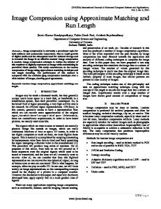
can provide the lowest compression rate (bit/pixel) as well as very high PSNR, which is larger than 46.37 dB. The average compression rate is 3.6 bits/pixel in seven standard test images when q=100%. Compared to the JPEG-LS near-lossless compression, the new algorithm improves about 23% compression rate as well as larger than 1 dB gain of PSNR. The experimental results also verify the theory analysis of (10). Note that when three components in Bayer data are compressed, respectively, the compression rate is lower only 3.4% than the proposed algorithm at the same PSNR. But the hardware overhead and power consumption of the proposed algorithm is much lower than that of the “G, B, and R respective compression method.” Compared with JPEG-LS lossless compression, although the proposed compression algorithm needs small hardware overhead of preprocessing part illustrated in Figure 13, the average compression rate of the proposed algorithm is lower 36% than that of JPEG-LS lossless compression. So the proposed compression algorithm is much better than JPEG-LS lossless compression for wireless endoscopy application. Table 3 also shows that the rounding operation can provide at least 3.5 dB gain of PSNR at the same compression rate. So the rounding operation is very important in this algorithm. Moreover, this algorithm can provide adjustable image quality and compression rate. When the quality control factor varies from 1 to 0, the relation between the PSNR and compression rate in three images, “airplane,” “lena,” and “baboon,” are illustrated in Figure 14. The columns to be filtered are always distributed equably in CFA raw data. In this figure, the PSNR is varied from 46.37 dB to infinity as well as the compression rate from 2.9 bits/pixel to 6.9 bits/pixel. The figure also shows that the more low-frequency contents there are in an image, the lower compression rate can be gotten. This near-lossless compression algorithm has been used in our designed wireless endoscopy system design. Six typical digestive tract images with 256 ∗ 256 size illustrated in Figure 15 are compressed with this algorithm. Table 4 shows that the proposed algorithm can provide higher compression performance than JPEG-LS near lossless compression (1) and (2). The average compression rate is about 2.12 bits/pixel with about PSNR 53.11 dB. The reason that the PSNR is larger than theoretical value, 46.37 dB, is that the images have been cut into a circle view and there is no rounding error in the black color location. The compression results in this table are better than Table 3 because the digestive tract images contain more low-frequency components. Note that the compression rate of the proposed algorithm is almost as same as that of the “G, B, and R respective compression method” at the same PSNR. So, this new near-lossless image compression algorithm is very suitable for the wireless endoscopy capsule system because the new algorithm makes full use of the characteristics of the medical images.
EURASIP Journal on Advances in Signal Processing
58 56 54 52 50 48 46 2.5
3
3.5
4
4.5
5
5.5
6
6.5
7
Compression ratio (pixel/bit) Baboon Lena Airplane
Figure 14: PSNR versus compression rate when the quality control factor varies from one to zero.
(a)
(b)
(c)
(d)
(e)
(f)
Figure 15: Six typical digestive tract images with 256 ∗ 256 size.
4.2. ASIC design implementation results The 0.18 µm CMOS process technology is used for the digital IC inside capsule. The digital IC photo is shown in
Figure 16. The die area is 3 mm ∗ 4.2 mm. Seven SRAMs are used to store the compressed image data (its maximum
Xiang Xie et al.
11 Table 4: Compression results for the six digestive tract images. CR means compression rate Image (256 × 256)
(a)
(b)
(c)
(d)
(e)
(f)
PSNR (dB)
53.121
53.103
53.100
53.135
53.083
53.128
CR(bits/pixel)
1.904
2.135
2.107
2.273
2.005
2.318
JPEG-LS near lossless
PSNR (dB)
51.3548
51.718
51.601
51.314
51.585
51.641
compression(1)
CR(bits/pixel)
2.7536
2.833
2.2784
3.302
2.489
2.892
JPEG-LS near lossless
PSNR (dB)
48.387
48.734
48.736
48.219
48.581
48.592
compression(2)
CR(bits/pixel)
2.168
2.411
2.189
2.631
2.063
2.415
G, B, and R respective
PSNR (dB)
53.132
53.111
53.101
53.135
53.083
53.129
compression method
CR(bits/pixel)
1.900
2.116
2.023
2.246
1.981
2.265
Proposed algorithm (q = 1)
SRAM
SRAM
SRAM
SRAM
Logical circuits
SRAM Dual port memory
consumption, the smallest area, and the shortest processing time. Therefore considering the tradeoff between the compression rate and the hardware expenditure, the proposed compression algorithm is more suitable for our wireless endoscopy system. 5.
SRAM
SRAM
Figure 16: Die photograph.
size is 640 ∗ 480 ∗ 2.4 = 92.16 KB) and JPEG-LS parameters with about 1.65 KB. One dual port block memory onchip is applied to store two line image data with 1.28 KB for image format transformation. The on-chip memory occupies about 70% area of the chip. The work clock frequency is 40 MHz. The power consumption shows that the total power consumption of the digital IC core is about 7.5 mW with 8 fps and 320 ∗ 288 image size or 2 fps and 640 ∗ 480 image size at 1.8 V. Table 5 shows the ASIC design comparison results of three different compression methods. The testing results of the proposed compression algorithm in Table 5 come from the real chip. The testing results of the other two compression algorithms are from the simulation by using the Synopsys tools such as Primetime, Astro, and DesignCompiler. The comparison results illustrate that the proposed compression algorithm has the lowest power
CONCLUSION
A low-complexity and highly efficient image compression algorithm suitable for ASIC design based on the Bayer format image applied in wireless endoscopy system has been presented. The reconstructed quality of seven standard color images can be changed from 46.37 dB to infinity as well as the compression rate which ranges approximately from 3.6 bits/pixel to 6.9 bits/pixel by adjusting the quality control factor. Furthermore, the average compression rate can reach 2.12 bits/pixel with the PSNR larger than 53.11 dB when the digestive tract images are compressed. Note that the new near-lossless compression algorithm provides lossless compression for the region of interest (ROI). Compared to the compression methods in which three components are compressed, respectively, although the proposed algorithm has 3.4% higher compression rate, from the hardware implementation viewpoint, it needs only two lines buffers, which is much simpler than those methods of G, R, and B respective compression. The VLSI architecture of the proposed compression algorithm has been implemented in 0.18 µm CMOS process. The experimental results show that the nearlossless image compression algorithm is suitable for the small size endoscopic capsule design with the requirement of lowpower, limited communication bandwidth and high image quality. It is also fit for on-chip CFAs of digital image sensor.
12
EURASIP Journal on Advances in Signal Processing Table 5: Comparison results of hardware cost, power dissipation, and processing time. Proposed compression algorithm
Serial compression structure
Parallel compression structure
Work clock frequency
40 MHz
40 MHz
40 MHz
Image size
640 ∗ 480
640 ∗ 480
640 ∗ 480
Logical gates
70 k gates
150 k gates
70 k gates
Memory consumption
93.81 KB + 1.28 KB
86.48 KB
195.84 KB
Power consumption
7.5 mW
19.2 mW
9.8 mW
Processing time
30.72 ms
30.72 ms
46.38 ms
Hardware area
12.6 mm2
14.7 mm2
23.1 mm2
ACKNOWLEDGMENTS This work is partly supported by the National Nature Science Foundation of China (no. 60372021) and partly supported by the National High Technology Research and Development Program of China (no. 2003AA1Z1100). REFERENCES [1] G. Iddan, G. Meron, A. Glukhovsky, and P. Swain, “Wireless capsule endoscopy,” Nature, vol. 405, no. 6785, pp. 417–418, 2000. [2] X. Xie, G. Li, X. Chen, et al., “A novel low power IC design for bi-directional digital wireless endoscopy capsule system,” in Proceedings of IEEE International Workshop on Biomedical Circuits and Systems (BIoCAS ’04), pp. S1.8-5–S1.8-8, Singapore, Republic of Singapore, December 2004. [3] Y. Ti. Tsai, “Color image compression for single-chip cameras,” IEEE Transactions on Electron Devices, vol. 38, no. 5, pp. 1226– 1232, 1991. [4] T. Toi and M. Ohita, “A subband coding technique for image compression in single CCD cameras with Bayer color filter arrays,” IEEE Transactions on Consumer Electronics, vol. 45, no. 1, pp. 176–180, 1999. [5] S.-Y. Lee and A. Ortega, “A novel approach of image compression in digital cameras with a Bayer color filter array,” in Proceedings of IEEE International Conference on Image Processing (ICIP ’01), vol. 3, pp. 482–485, Thessaloniki, Greece, October 2001. [6] C. C. Koh, J. Mukherjee, and S. K. Mitra, “New efficient methods of image compression in digital cameras with color filter array,” IEEE Transactions on Consumer Electronics, vol. 49, no. 4, pp. 1448–1456, 2003. [7] S. Battiato, A. Buemi, L. Della Torre, and A. Vitali, “A fast vector quantization engine for CFA data compression,” in Proceedings of IEEE-EURASIP Workshop on Nonlinear Signal and Image Processing (NSIP ’03), Grado, Italy, June 2003. [8] N. Zhang and X. Wu, “Lossless compression of color mosaic images,” in Proceedings of IEEE International Conference on Image Processing (ICIP ’04), vol. 1, pp. 517–520, Singapore, Republic of Singapore, October 2004. [9] B. E. Bayer, “Color imaging array,” US patent no. 3,971,065, 1976. [10] M. J. Weinberger, G. Seroussi, and G. Sapiro, “The LOCOI lossless image compression algorithm: principles and standardization into JPEG-LS,” IEEE Transactions on Image Processing, vol. 9, no. 8, pp. 1309–1324, 2000.
[11] X. Wu, “Lossless compression of continuous-tone images via context selection, quantization, and modeling,” IEEE Transactions on Image Processing, vol. 6, no. 5, pp. 656–664, 1997. [12] P. G. Howard and J. S. Vitter, “Fast and efficient lossless image compression,” in Proceedings of the IEEE Data Compression Conference (DCC ’93), pp. 351–360, Snowbird, Utah, USA, April 1993. [13] X. Xie, G. Li, C. Zhang, and Z. Wang, “An efficient control strategy of adaptive packet length for ARQ in wireless endoscopy system,” in Proceedings of International Symposium on Communications and Information Technologies (ISCIT ’05), vol. 2, pp. 1121–1123, Beijing, China, October 2005. [14] S. W. Golomb, “Run-length encodings,” IEEE Transactions on Information Theory, vol. 12, no. 3, pp. 399–401, 1966.
Xiang Xie was born in Hunan province, China, in 1971. He received his B.S. and M.S degrees from Navy Electronic Engineering College in 1993 and 1996, respectively. He is currently working towards his Ph.D. degree at the Tsinghua University, Beijing, China. His research interests include wireless communication, image processing, biomedical electronics, and digital IC design. GuoLin Li received his Bachelor’s, Master’s, and doctor degrees from the Electronic Engineering Department of Tsinghua University in 1993, 1998, and 2002, respectively. Now he is a Lecturer of Tsinghua University. From 1993 to 1996, he had participated in a 1.8 GHz-transceiver design for digital microwave communication. His current research interest is the analysis of interconnections and design of RFICs. ZhiHua Wang was born in Shandong province, China, in 1960. He received the B.S., M.S., and Ph.D. degrees from the Department of Electronic Engineering, Tsinghua University, Beijing, China, in 1983, 1985, and 1990, respectively. He became a Professor in the Department of Electronic Engineering and Vice Director of the Institute of Microelectronics of Tsinghua University in 1997 and 2000, respectively. He has served as the official Member of the Commission C of China
Xiang Xie et al. National Commission of URSI starting 1998 and the Chairman of the IEEE Solid-State Circuit Society Beijing Chapter. His major research fields are the design methodology and design automation of integrated circuits and systems, design of integrated circuits for communication, and high-speed real-time signal processing.
13