In order to achieve a balance between design quality and time-to-market, cell library based design is becoming the dominant design methodology over the ...
A Network-Flow Based Cell Sizing Algorithm Huan Ren and Shantanu Dutt Dept. of ECE, University of Illinois-Chicago Abstract—We propose a timing-driven discrete cellsizing algorithm that can incorporate total cell size constraints. We model cell sizing as a min-cost network flow problem. In the network flow graph, available sizes of each cell are modeled as nodes. Flow passing through a node indicates the choice of the corresponding cell size, and the total flow cost reflects the timing objective function value change with the chosen sizes of cells. Compared to other discrete optimization methods for cell sizing, our method can obtain a near-optimal solution in a very timeefficient manner. We tested our algorithm on the ISCAS’85 benchmark, and compared our results with an optimal solution produced by an exhaustive search method with exponential time complexity. The results show that given the same initial sizing, the improvement obtained by our method is only 1% worse (11.9% v.s. 12.9%) than the optimal solution, while satisfying a given total cell area constraint. Furthermore, our method is 60 times faster than the optimal method.
1. Introduction In order to achieve a balance between design quality and time-to-market, cell library based design is becoming the dominant design methodology over the custom design method even for high performance ICs. Usually in a cell library, several different cell implementations are available for the same function with different sizes, intrinsic delays, driving resistances and input capacitances. Choosing the cell with an appropriate size, i.e., cell sizing, is a very effective approach to improve timing. The cell sizing problem has been studied for a long time. Many methods [5], [8] assume the availability of a continuous range of cell sizes, i.e., the size of a cell can take any value in a range. Then, the obtained gate size is rounded to the nearest available size in the library. However, a large number of realistic cell libraries are “sparse”, e.g., geometrically spaced instead of uniformly spaced [9]. Geometrically spaced gate sizes are desired in order to cover a large size range with a relatively small number of cell instances. Also it has been proved in [4] that under certain conditions, the set of optimal gate sizes must satisfy the geometric progression. With a sparse library, the simple rounding scheme can introduce huge deterioration from the continuous solution, which often causes the sizing results to fail to meet given timing requirements [9]. On the other hand, few time-efficient methods are know that can directly handle timing optimization with discrete cell sizes, since this problem is NP-complete. The technique in [6] uses multi-dimensional descent optimization, that iteratively improves a current solution by changing the size choices of a set of cells that produces the largest improvement. It is not clear how well this method can avoid being trapped in a local optimum. In [9], a new rounding method is developed based on an initial continuous solution. Instead of only rounding to the nearest available size, it visits cells in topological order in the This work was supported by NSF grant CCR-0204097.
circuit, and tries several discrete sizes around the continuous solution for each cell. In order to reduce the search space, after a new cell is visited, it performs a pruning step that discards obviously inferior solutions, and a merging step that keeps only several representative solutions within a certain quality region. The run time of this method is significantly larger than the method in [6]. In this paper, we propose a network-flow based method for the discrete gate-sizing problem. In our method, the different size options of a cell are modeled by nodes in the network graph. The flow cost represents the change in the timing objective function value when the cell sizes corresponding to the nodes in the graph that have flows through them are chosen. Hence, by solving a min-cost flow in the network graph, nearoptimal cell sizing can be determined by choosing cell sizes whose corresponding nodes have the min-cost flow through them—the near-optimality comes from having to constraint the flow to adhere to certain discrete requirements like going through exactly one size-option node per cell. By modeling the gate-sizing problem as a min-cost network flow problem, we can solve it using standard network flow algorithms, which are very time efficient. Also problem constraints like the maximum allowable total cell area, can be handled efficiently by making the flow amount proportional to the chosen cell area, and using an arc with an appropriate capacity to limit the total flow amount. However, network flow is a continuous optimization method. Thus when applying it to solve the discrete option selection problem, invalid solutions may be produced. For example, the min-cost flow may pass through two sizing options for the same cell. We solve such problems by using min cost or max flow selection heuristics. The rest of the paper is organized as follows. Section 2 provides an overview of our method. A general view of our size selection network graph (SSG) is presented in Sec. 3. In Secs. 4-7, we discuss various issues of the SSG. In Sec. 8, we show how to obtain a valid min-cost flow in the SSG. Section 9 briefly describes an optimal exhaustive search method to which we compare our network-flow based technique. Section 10 presents experimental results and we conclude in Sec. 11.
2. Overview of Our Method Our cell sizing method starts from an initial sizing solution that may be far from the optimal. The objective is to improve the critical path delay of the circuit by resizing cells. We define Pα to be the set of paths with a delay greater than 1−α fraction (α < 1) of the most critical path delay. In order to reduce the complexity of the problem we only consider changing the sizes of cells in Pα . In our experiments, α is set to be 0.1. This simplification does not limit the optimization potential of our method, since our method is incremental in its nature. Thus we can iterate it several times to take more paths into consideration. We define CS(nj ) to be the set of critical sinks of a net n j , which are: 1) all sinks in Pα if the net is in Pα , or 2) the sink with the minimum slack otherwise. Our method tries
n3
n1
n7 n5
1
n2
f n4
n6 (a)
Net structure
N1
uk ud
Net spanning structure
uj
N5
S (Source)
N2
N4
cap=total area contraint
Area gathering node (b)
Fig. 1. (a) Nets in Pα of a circuit. (b) The corresponding SSG, which includes net structures and net spanning structures. Ni is the net structure corresponding to net ni . Each net structure will send a flow of amount equal to the total cell size it chooses through the area output arc to the area gathering node. All these flows are routed to the sink through an arc from the area-gathering node with a capacity equal to the given total cell area constraint.
to improve the critical path delay by minimizing the objective function proposed in [7]. A timing cost tc (ni ) of a net ni is defined as [7]: tc (ni ) =
∑
β
D(u j , ni )/Sa (ni )
(1)
where u j is a sink cell of net ni , D(u j , ni ) is the net delay of ni to u j , and Sa (ni ) is the allocated slack of a net in the initial sizing solution; the allocated slack is defined as the path slack divided by the number of nets in the path. β is the exponent of the allocated slack used to adjust the weight difference between costs of nets on critical and non-critical paths. Based on experimental results, β = 1 works best in this scenario, since only nets in Pα and those connected to it are considered in the optimization function (see below). Let Pˆα be the set of nets that are either in Pα or connected to nodes in it. The timing objective function Ft is the summation of tc (ni ) of all nets in Pˆα given as:
∑
1 Su j
Su d
2
(b)
to one sizing option. We use flows in the SSG to model cell size selection, i.e., a size option of a cell is chosen by a flow in the SSG if its corresponding option node in the SSG is on the path of the flow. Hence, each flow through the SSG that passes through one option node in every set of sizing options in the SSG corresponds to a sizing selection for the cells in Pα . Furthermore, if we can set the costs of arcs between option nodes in the SSG in such a way that the total cost incurred by a flow through the SSG is equal to the change in the timing objective function Ft (Eqn. 2) corresponding to the sizing scheme selected by the flow, then the min-cost flow in the SSG selects the optimal cell sizing scheme for Ft . Hence the problem of finding the optimal cell sizing is converted to the problem of finding the min-cost flow in a graph for which several efficient algorithms such as the network simplex algorithm and the enhanced scaling algorithm [2] are available. The general structure of our SSG is described below.
A. The SSG Structure
u j ∈CS(ni )
Ft =
2
Su k
Fig. 2. (a) A net in critical paths. (b) The net structure corresponding to the net; f is a flow through the net structure.
T (Sink)
N6
Area output arcs
Complete bipartite subgraph
(a)
N7
N3
2
1
tc (ni )
(2)
ni ∈Pˆα
Here we only consider nets in Pˆα , since the delays of only these nets will change with our selection of resizable cells. Note that in this objective function the nets on more critical paths have a higher contribution since the net cost is inversely proportional to the allocated slack, and thus will be optimized more—a desirable outcome, especially in a scenario where there is a quota on the resource (e.g. total area) available for optimization. Usually, the total area is given as a constraint for timing driven cell sizing. Our algorithm can also handle this constrained optimization problem.
3. The Size Selection Graph (SSG) We model the timing-minimization cell size selection problem as a min-cost network flow problem. A network flow graph called the size selection graph (SSG) is constructed in which the set of sizing options of each cell is modeled as a set of sizing option nodes, and each sizing option node corresponds
Since Ft is the summation of the timing costs tc of nets, we employ a divide-and-conquer approach in constructing the SSG, i.e., first a mini network flow graph called a net structure is constructed for each net in Pα , and then net structures of connected nets are connected by net spanning structures to form the complete SSG as shown in Fig. 1. Thus, the SSG has a similar topology as the paths in Pα . A net structure N j is a child net structure of Ni if they are connected and N j follows Ni in the flow direction in the SSG (i.e. the signal direction in the circuit is from net ni to net n j ); correspondingly Ni is also a parent net structure of N j . Each net structure contains the sets of option nodes for cells in the corresponding net. Let us denote the set of sizing options of a cell u as Su , and the l’th sizing option in it as Sul . For a net ni with a driving cell ud , the net structure is constructed by connecting each sizing option Sul d of ud to all sizing option nodes in Suk of every sink cell uk to form a complete bipartite subgraph between Sud and Suk . An example is shown in Fig. 2. The net has one driving cell ud and two critical sink cells u j and uk ; see Fig. 2(a). The corresponding net structure is shown in Fig. 2(b). Here, we only show two sizing options in each option set. A flow f through the net structure is also shown, which selects size option Su1d for ud , Su1k for uk and Su2 j for u j . With the complete bipartite subgraphs between the sizing option sets of the drive cell and sink cells in a net structure, every possible combination of size choices of cells in the net has a corresponding flow through the net structure, and hence is considered in our size selection process. There are two major issues that need to be tackled in constructing the SSG in order to correctly map the min-cost flow in the SSG to an optimal sizing choice. These are: (1) In each net structure, the cost of each arc needs to be determined so the total cost of a flow through the net structure can accurately capture the change value of the timing cost tc
for the net corresponding to the sizing options chosen by the flow. A detailed description of this issue is given in Sec. 4. (2) The flow that is determined must be a valid flow, i.e., can be converted to a valid sizing option selection. A valid sizing option selection requires the satisfaction of two types of consistencies. First, sizing option nodes of a particular cell has to be chosen in a mutually exclusive manner (consistency in a sizing option set). Second, if a cell is connected to multiple nets, its sizing options will also be included in each of the corresponding net structures. In such cases, the selected sizing options for the cell must be consistent across all these net structures (consistency across net structures). As described in Sec. 5, the net spanning structure is designed to guide flows between net structures in the SSG to satisfy the second type of consistency. To guarantee the first type of consistency, two heuristic methods are proposed that prune flows corresponding to invalid option selections when determining the min-cost flow; these are discussed in Sec. 8.
B. Handling the Area Constraint To handle any given total cell area constraint, each net structure has an outgoing arc called the area output arc. A shunting structure as explained in Sec. 6 is present in each net structure and connects the area output arc with the option nodes in the net structure. The function of the shunting structure is that when an option node is chosen, the shunting structure will diverts a flow of amount that equals to the chosen size to the area output arc from the incoming flow to the option node. All these flows are gathered at the area gathering node as shown in Fig. 1(b) which is connected to the sink. By setting the capacity of the arc between the area gathering node and the sink to be the given total cell area limit, we make sure the total selected cell area, which is equal to the total incoming flow amount to the area gathering node, is smaller than or equal to the given limit. The shunting structure is discussed in detail in Sec. 6. Note that as mentioned before, the sizing option of a cell can be contained in more than one net structure; in this case, the flow amount equal to its selected area will be sent to the area output arc in only one of the net structures that contains the cell. The high-level pseudo code of our cell sizing method FlowSize is given in Fig. 3.
4. Arc Cost Determination To explain our arc cost formulation that accurately captures the timing cost change, we assume a lumped capacitance and resistance net delay model, which is widely used in cell sizing [4], [8], [10]. For net ni , the delay D(u j , ni ) to a sink cell u j of ni is: D(u j , ni ) = Rd (c · Lni +
∑
Cuk )
uk ∈SC(ni )
where Rd is the driving resistance of ni , c is the unit WL capacitance, Lni is the WL of ni , SC(ni ) is the set of sink cells of ni , and Cuk is the input capacitance of cell uk . In the pre-placement sizing stage, the WL of a net is usually estimated according to the fan-out number of the net. In the post-placement resizing stage, it can be estimated using one of several well know models, e.g., HPBB. With this delay model, for a critical net ni with m critical sinks, the timing cost tc (ni ) of ni is: tc (ni ) =
m β Sa (ni )
· Rd (c · Lni +
∑
uk ∈SC(ni )
Cuk )
Algorithm FlowSize 1. Construct a net structure as depicted in Fig. 2 for each net in Pα . 2. Determine the cost of each arc in the net structures, so that the change in timing cost is accurately incurred by flows through them. 3. Connect net structures with net spanning structures that maintain consistency of size selection of common cells across multiple net structures; see Sec. 5. 4. Add the shunting structure and an area output arc (Sec. 6) to each net structure to divert flow of amount equal to the selected size options (nodes) to the area output arc. 5. Connect area output arcs to the area gathering node that has only one outgoing arc with capacity equal to the area constraint to limit total selected cell area (= flow amount into the node). 6. Determine a valid min-cost flow in the resulting SSG by applying the standard min-cost flow algorithm and the min-cost/max-flow heuristics (Sec. 8) iteratively. 7. Select the size options chosen by the valid min-cost flow as cell sizes to obtain a near optimal critical path delay for the circuit. Fig. 3. Network flow algorithm for the cell sizing problem for optimizing timing under a given area constraint.
In the above expression, let us denote the coefficient βm Sa (ni ) as α. The parameters affected by cell sizing options are Rd and Cuk . Hence, if a term in the formula includes Rd , its value is determined by the size of ud , and if a term includes Cuk , its value is determined by the size of uk . For example, the term αRd ·Cuk is determined by choices in sizes of both ud and uk , and the value change of this term ∆ αRd Cuk (Sul d , Sumk ) when the two sizing options Sul d and Sumk are chosen can be written as: ∆ αRd Cuk (Sul d , Sumk ) = α[Rd (Sul d ) ·Cuk (Sumk ) − Rd (Su� d ) ·Cuk (Su� k )] where Rd (Sul d ) is the driving resistant corresponding to the driver cell ud with size option Sul d , Cuk (Sumk ) is the input capacitance of uk with size option Sumk , and Su� d and Su� k are the original sizes of ud and uk , respectively. The term αRd · c · Lni is determined only by the size of ud , and its value change ∆ αRd cLni (Sul d ) when the option Sul d is selected is: ∆ αRd cLni (Sul d ) = α · c · Lni (Rd (Sul d ) − Rd (Su� d )) We denote the set of arcs between Sud and Suk as E(Sud , Suk ), where ud is the driving cell, and uk is a sink cell. A valid flow will pass through only one arc in each such arc set, since only one option in Sud and Suk can be meaningfully chosen. Hence, in order to make the valid flow cost equal to the change of the timing cost, the cost of an arc in an arc set is set as the sum of the changes of all terms in the timing cost function that are functions of the cell size options represented by the arc. Furthermore, if a term in tc is a function of only the size of one cell v, then we arbitrarily choose an arc set E(Sv , Sw ) among all those connected to Sv , and the term value change determined by each Svl is added to all arcs starting from option node Svl in the arc set. Thus, the value change of term αRd Cuk is included in the cost of the arc set E(Sud , Suk ). Specifically, the cost of an arc (Sul d , Sumk ) in the set includes ∆ αRd Cuk (Sul d , Sumk ). The value change of term αRd c · L(ni ) is a function only of the driving cell size, and thus is included in the cost of arcs in only one arc set E(Sud , Su j ), where u j is an arbitrary chosen sink cell of
ni . Specifically, the cost of an arc (Sul d , Sumj ) in the set includes ∆ αRd cLni (Sul d ). Finally, the size change of a cell in a critical net also affects the timing cost of non-critical nets that are connected to the cell. Instead of also constructing net structures for these affected non-critical nets, we use a much simpler method, which is including the timing cost changes of non-critical nets in the net structures of their connected critical nets. Let u be a cell in Pα . We have two cases w.r.t. u and any non-critical net (a net not in Pα ) it may be connected to: (1) If u is the driver of a non-critical net n j , the timing cost β change of n j is (Rd (Sul ) − Rd (Su� ))(c · Ln j +Cload (n j ))/Sa (n j ), l � where Su is the chosen option of u, Su is the initial size of u, and Cload (n j ) is the total load capacitance of n j . (2) Otherwise, if u is a sink cell of a non-critical net n j , β the timing cost change of n j is Rd (Cu (Sul ) −Cu (Su� ))/Sa (n j ). u l Let ∆ tc (Su ) denote the total timing cost change of all noncritical nets connected to u. If u = ud is the driving cell of the critical net ni , ∆ tcu (Sul ) is included in arcs in one arc set E(Sud , Su j ), where, again, u j is the arbitrarily chosen sink cell of ni . Otherwise, if u = uk is a sink cell, ∆tcu (Sul ) is included in the arc set E(Sud , Suk ). Specifically, the cost of an arc (Sumd , Sul k ) includes ∆ tcu (Sul ). To sum up, for an arc (Sul d , Sumk ) in a net structure, if uk = u j (u j is the chosen sink in whose arc set E(Sud , Su j ) cost, i.e., costs of the arcs in this set, we include the change in the terms in Ft that are only dependent on the cell size of driver ud ), its cost cost(Sul d , Sumk ) is: cost(Sul d , Sumk )
=
∆ αRd Cuk (Sul d , Sumk ) + ∆ αRd cLni (Sul d )
+
∆ tcud (Sul d ) + ∆ tcuk (Sumk ).
Otherwise if uk �= u j , its cost is: cost(Sul d , Sumk ) = ∆ αRd Cuk (Sul d , Sumk ) + ∆ tcuk (Sumk ).
5. Maintaining Consistency Across Net Spanning Structures As we mentioned before, the net spanning structure is designed to maintain consistency across net structures. Note that if multiple nets have a common cell, their net structures must be connected in the SSG by net spanning structures. We first consider the situation in which a cell u is a sink cell of a net ni , and the driving cell of k nets n j1 , . . . , n jk (k ≥ 1); see Fig. 4(a). The size option set Su is present in all the net structures corresponding to these connected nets. We connect these net structures by adding arcs from each option node in Su of Ni to the equivalent option node (indicating the same size choice) in the Su ’s of N j1 , . . . , N jk , where Ni is the net structure corresponding to net ni . The resulting spanning structure is shown in Fig. 4(b). With this structure, it is easy to see that if one size option of u is chosen by the flow through Ni , then this flow will also pass through the equivalent option nodes in N j1 , . . . , N jk . Thus, the required consistency is maintained. The other situation is that the common cell u is the sink cell of more than one net ni1 , . . . , nil (l > 1) and the driver of at least one net n j , as shown in Fig. 4(c). In this situation, we will treat each Nim (1 ≤ m ≤ l) individually, and make the connections between each Nir and N j as stated in the first situation. However, in this case the spanning structure cannot guarantee the consistency of the option selected for
u
ni
n j1
n i1
n j2
n i2
(a)
(c) Su
Su 1
Ni
Nj1
Ni1
1 2
2
1
u nj
1
Nj
2
2
1
Su
(b)
1 Nj2
Ni2
2
2
Su
Su
Su
(d)
Fig. 4. The net spanning structure. (a) The common cell u is a sink cell of one net ni , and the driver of multiple nets n j1 and n j2 . (b) The corresponding spanning structure of [a], where Nk is the net structure corresponding to net nk . (c) u is a sink cell of multiple nets ni1 and ni2 , and the driver of n j . (d) The corresponding spanning structure of [c].
u in Ni1 , . . . , Nil . We use a min-cost heuristic to tackle this problem; this is described in Sec. 8. The costs of all arcs in the spanning structure are 0.
6. Tackling the Cell Area Constraint As we mentioned before, for each net structure, there is an area output arc. cap= A(Sul d ) cap= A(Sumk ) Once a sizing option node is chosen, a flow with an f amount equal to the chosen Sumk size needs to be sent to this l Su d arc—this flow is then sent Net structure to the sink via a common Fig. 5. Flows to the area output arc area-gathering node and its of a net structure. capacity-constrained arc in order to satisfy the total cell area constraint. The simplest way to achieve this is adding to each option node an arc leaving the net structure to the area output arc with a capacity equal to the option size. Then if enough flow comes into the option node, the desired amount will be sent to the area output arc. An example is shown in Area output arc Fig. 5. A flow f selects two cap=A(Sul ) sizing options Shunting l cap=Amax(S u)− A(S u) node Sul d and Sumk and incurs the cap=Amax(S u) Sink Leaving corresponding arc cost of arc Slu (Sul d , Sumk ) in a net Flow from the structure. A(Sul ) net structure is the size of an option Sul . At Fig. 6. The shunting structure for outgoing each of the two flows from a net structure. option nodes, a branch of flow diverges a part of f to the area output arc with amount equal to the corresponding option sizes. However, with this structure, the amount of flow that leaves a net structure is dependent on the option selected, and is thus a variable. This is not desirable for determining the capacities Area output arc
of arcs in the spanning structures—the capacities of arcs in a spanning structure from net structure Ni to N j needs to be a constant, i.e., independent of the size choices made in Ni by the flow entering Ni . We thus need a structure to diverge a constant amount of the flow that enters Ni ; this amount is ∑u∈ni Amax (Su ), where Amax (Su ) is the maximum size of options in Su . Our complete structure for diverging flows to the area output arc is shown in Fig. 6. In the structure, the capacity of the arc leaving towards the sink (called the leaving arc) from each option node in an option set Su is set to be Amax (Su ). Therefore, the amount of flow leaving the net structure from any option node ∈ Su is always Amax (Su ). However, not all this amount is sent to the area output arc. A shunting node is connected to each of these leaving arcs, and divides the flow into two parts, one to the area output arc, and the other one shunted (i.e., sent directly) to the sink. If the leaving arc is from an option node Sul , the capacity of the arc between the shunting node and the area output arc is then A(Sul ), and the capacity of the arc to the sink is Amax (Su ) − A(Sul ). Therefore, if Sul is chosen, the amount of flow sent to the area output arc is exactly A(Sul ), and the rest of the amount Amax (Su ) − A(Sul ) is shunted to the sink. In this way, we send the correct amount of flow into the area output arc of each net structure Ni , and also make the total amount of flow leaving Ni to the sink be ∑u∈ni Amax (Su ). The costs of all arcs in this structure between an option node and the area output arc are 0.
7. Capacity Determination Setting proper capacities for arcs is very important for the correct functioning of the SSG. The capacities should be set such that: 1) sufficient flow can be sent to each net structure in the SSG to meet the flow demand on its area output arc; 2) within a net structure, the total incoming flow can be distributed to all sink and the driver cell option sets. In order to determine the arc capacity, we first determine how much incoming flow is needed for each net structure. A net structure has two types of outgoing flows: 1) into the area output arc for area constraint satisfaction; 2) supply flow to its child net structures. The first type of outgoing flow has a fixed amount ∑u∈ni Amax (Su ) for a net structure Ni , irrespective of the chosen sizing options, as discussed in Sec. 6. The incoming flow amount must be sufficient to cover the two outgoing flows, and thus the required incoming amount fin (Ni ) of a net structure Ni is recursively given as: fin (Ni )
=
∑ Amax (Su ) +
u∈ni
fin (Ni )
=
∑
fin (N j )/din (N j )
Nj ∈child(Ni )
if Ni has any child net structure ∑ Amax (Su ), u∈ni
(3) otherwise (Ni is a ”leaf” net structure in the SSG) where child(Ni ) is the set of child net structures of Ni , and din (N j ) is the incoming degree of N j , i.e., the number of parent net structures of N j . In Eqn. 3, we assume that the required flow amount for a net structure is sent uniformly from all its parent net structures. The determination of the flow needed in each structure starts from the boundary condition of “leaf” net structures given in Eqn. 3 that are directly connected to the sink. The incoming flow amount needed for these net structures is the total of their first type of outgoing flows. Starting from the leaf net structures, we visit other net structures in a reverse
topological order and determine their required incoming flow amount according to the formulation in Eqn. 3. After obtaining fin for each net structure, we can determine its arc capacities as follows: • For an arc in the net spanning structure from Ni to N j , its capacity is fin (N j )/din (N j ), which equals the flow amount sent from Ni to N j according to Eqn. 3. This makes the total incoming flow amount to a net structure Ni exactly fin (Ni ). As mentioned before, the cost of this arc is 0. • Within a net structure, the capacities of arcs in each arc set E(Sud , Suk ) are the same and is derived below; ud is the driving cell and uk is any sink cell of the corresponding net. For an arc set E(Sud , Suk ), if Suk is not connected to any arc in the outgoing spanning structure of Ni , the capacity of each arc in it is set as Amax (Suk ), so that sufficient flow can be sent to the leaving arc for constraint satisfaction. Otherwise, let N j1 , . . . , N jt be the child net structures of Ni that Suk is connected to (via spanning structures). Note that this means that uk is a common cell in nets ni and n j1 , . . . , n jt . Then, the capacity of each arc in the set is set to be Amax (Suk ) + ∑tr=1 fin (N jr )/din (N jr ).
A. Unit Flow Arc Cost When we gave the costs of arcs in a net structure in Sec. 4, we assumed that any flow on the arc will incur the cost. However, in a standard network flow graph, the cost of a flow on an arc is determined as the flow amount multiplied by the unit flow cost of the arc. With the above capacity assignment, a valid flow will always be a full flow on each arc it passes through in a net structure, since the summation of the arc capacity of a single arc in each arc set is equal to the incoming flow amount, and a valid flow uses exactly one arc in each arc set. In order to incur the same cost for a valid flow as determined in Sec. 4, the unit flow cost C(Sul d , Sumk ) of an arc (Sul d , Sumk ) is set to be the corresponding arc cost given in Sec. 4 divided by its capacity as determined above, i.e., C(Sul d , Sumk ) = cost(Sul d , Sumk )/cap(Sul d , Sumk )
8. Finding a Valid (Discretized) Min-cost Flow The standard min-cost network flow 2 2 solves a linear S um S um d d programming Su Su k k problem (a (a) (b) continuous Fig. 7. (a) Invalid flow f through two sizing options of the same cell uk . (b) Selecting only optimization one option of Suk for the next iteration based on method). Hence, it cannot some criteria of the previous “split flow”. automatically handle the consistency (mutual exclusiveness) requirement in a size option set for a particular cell, which may result in an invalid min-cost flow for size selection. Therefore, after one iteration of a min-cost network flow process, in a net structure, the obtained min-cost flow may pass through an option node Sumd for the driving cell ud and then to two or more sizing options in Suk for a sink cell uk as shown in Fig. 7(a). Furthermore, as explained in Sec. 5, the resulting flow may also violate the consistency requirement for the size option selection across net structures that have a common sink cell. f
1
1
Su
Su
f1
1
1
S vm S wl
2
f2
1 2
1 2 Su
(a)
Su Net structures
S vm S wl
1
2
2 1
Su
2
Net structures
Su
(b)
Fig. 8. (a) Inconsistent option selections of the same cell u in different net structures. f1 chooses option Su1 ; f2 chooses option Su2 . (b) The same option Su1 of u is selected in the next iteration for all net structures contains u as a sink cell based on some criteria of the previous flow of [a].
In the above two cases, we will start a new iteration of the network flow process by pruning out some options that lead to an invalid flow based on certain criteria of the flow so that a near-optimal size selection is obtained. In the new iteration, for the first case, Sumd will only connect to one of the option nodes in Suk that had flow through them in the first iteration as shown in Fig. 7(b); the selection criterion is discussed shortly. Similarly for the second case, in all net structures whose corresponding nets have u as a sink cell, the chosen driving cell options in the first iteration, e.g., Svm and l as shown in Fig. 8(b), will only connect to the same sizing Sw option of u selected from those that had flow through them in the first iteration. In this way, the same invalid flow will not occur in the second iteration. We have used two alternative selection heuristics to choose a good option node from a illegal selection in each option set Su to be part of the new iteration: • Max-flow heuristic: Always choose the option node with the largest flow amount through it. • Min-cost heuristic: For the first situation, starting from Sumd , follow the path of each branch of the min-cost flow up to a length of l, and choose the option node that is on the branch that has the min-cost path. For the second situation, for each currently selected option of u, the cost that we use to determine whether it is a good option consists of two parts, output path cost and incoming arc cost. As shown in Fig. 9, similar to the first situation, the outgoing path cost of an option Sul of u is the cost of the flow path starting from the option node. The incoming arc cost of an option Sul of u is the total cost of the set of incoming arcs G(Sul ) to all Sul ’s across all net structures that contain the option set Su ; see Fig. 9. The summation of these two costs is a good estimation of the cost of a valid flow that chooses only option Sul for cell u. Hence, we choose the option with smallest summation of the path cost and the arc cost. Note that due to run time consideration we cannot always follow each branch flow to the sink. We thus set a limit l (in number of net structures) on the length of paths we follow. The percentage timing improvement of four representative circuits in Table I for the ISCAS85 benchmarks reveals that the min-cost heuristics with path length limits of 2, 3, 4, and 5 perform consistently better than the max-flow heuristic, and have a relatively better performance in the range of 24-39%. The min-cost heuristic is thus implemented in our algorithms, and we set l = 3 for a balance between computational complexity and accuracy.
Ckt
Max-flow
C432 C1355 C3540 C7552 avg.
%∆ T 8.4 4.2 12.9 8.3 8.4
Min-cost of length 2 3 4 5 %∆ T %∆ T %∆ T %∆ T 10.0 11.9 12.2 12.2 6.0 6.8 6.9 7.2 16.1 16.8 17.0 17.1 9.3 9.9 10.3 10.5 10.4 11.4 11.6 11.7
TABLE I Percentage timing improvements of max-flow heuristic and min-cost heuristic with different path length limits.
A. Time Complexity of FlowSize It is easy to see that with the two pruning heuristics, if the option selection for a cell is inconsistent according to the mincost flow obtained in one iteration, in the following iterations the min-cost flow will select a valid size option for the cell. Thus, the number of iterations required to reach a valid mincost flow is no more than the total number of cells in Pα . In each iteration, Flow path we use the network Su simplex algorithm to solve the min1 f1 cost flow. Given a 1 graph with m arcs, 2 S vm if the capacities and 2 1 G( Su ) costs of arcs are 1 Su all integers, with U l Sw being the maximum 2 arc capacity and C Su being the maximum Fig. 9. The flow path for determining arc cost, then the 1 the path cost of Su , and the arcs for time complexity of 1 determining the arc cost of Su . the network simplex method is O(Um2 logC) [3]; however, it is well-known that the average-case run time of the simplex method is much lower than this worst-case complexity [1]. As described in Sec. 7, the capacities of arcs in our SSG, being the summation of cell sizes, are integers (note that cell sizes in a standard cell design are integer in the unit of the technique feature size of the library). On the other hand, while our cost is not integer, it can be converted to integer values by proper scaling. Hence though we do not actually do the scaling, we use this assumption here in order to derive an upper bound on the time complexity of our algorithm. Let us first consider the total number of arcs in our SSG. It is dependent on the number of cells N, the number of nets M in the circuit, and the number of available sizes for each cell S. There are three types of arcs in our SSG: arcs between size option sets, arcs in net spanning structures, and arcs in shunting structures. The number of arcs between two size option sets is S2 , and in each net structure there are d − 1 sets of such arcs, where d is the degree of the corresponding net. Thus, the total number of these arcs in the SSG is S2 (davg − 1)M, where davg is the average degree of nets in a circuit. Since davg is usually no more than 4, the total number of arcs between size option sets is O(S2 M). The number of arcs in the shunting structure for each option node is three, and hence the total number is 3NS. The net spanning structure only connects size option sets for the same cell in multiple net structures, and the number of arcs between two of such size option sets is S. Since the total number of size option sets is O(N), the total number of arcs in the net spanning structure is thus O(NS). To sum up, the total number of arcs in the SSG is O(S2 M + NS). The maximum arc capacity is equal to the total cell size when all cells are chosen to be at their maximum width, and
Ckt
thus is O(N). The maximum arc cost is less than or equal to the maximum net delay. The delay of a net is dependent on the driving resistance of the driving cell, input capacitances of the sink cells and the net fanout. Since the driving resistances and input capacitances of cells are constants specified by the library, and the average fanout is usually a small constant in a VLSI circuit, C can be viewed as a constant. Typically in a real circuit, N and M are about the same. Hence, the number of arcs in our SSG can be rewritten as O(S2 N). Therefore, the time complexity of each iteration is O(S4 N 3 ), and the total time complexity is then O(S4 N 4 ). The polynomially bounded time complexity is a highlight of our algorithm FlowSize, since other discrete cell sizing methods such as [6], [9] are not polynomially bounded in run time. Also, as we show in Sec. 10 (Fig. 11), its actual run-time reveals a much smaller complexity that is in keeping with the much smaller average-case run time of the network simplex algorithm compared to its worst-case complexity. Furthermore, our experiments show that the actual number of iterations needed in FlowSize is much less than the number of cells in Pα , e.g., eight iterations for a circuit with 300 cells in Pα .
9. An Optimal Exhaustive-Search Algorithm Since we do not have the library or library parameters used in [9], we cannot directly compare to their technique. Thus, we implemented an exhaustive search method that can produce optimal solutions for the sizing problem of cells in Pα , and compare our solution quality to the optimal one. The idea of this exhaustive search is to try every possible cell sizing solution, and choose the one with best critical path delay. However, if no proper solution pruning method is applied, the run time of the search would be unacceptable even for the smallest circuit in the benchmark. We propose three pruning methods that can maintain the optimality of the solution, but greatly reduce the run time. In the exhaustive search method, we visit cells in topological order, and when we are visiting a cell, we will combine all partial solutions we have for all visited cells with possible size choices of the current cell to form new partial solutions. The pruning process happens after new partial solutions are generated. We propose three pruning unvisited cells visited cells conditions. A partial ...... ck ...... cj solution is output input pruned when: boundary 1) it fails to meet the area Fig. 10. Visited cells, unvisited cells and the constraint; 2) it gives longer boundary between them. delay than the critical path delay produced by our method; 3) there is another better partial solution (generated in the search process or extracted from the complete solution of our method) that gives smaller total area, and better arrival time at the outputs of cells on the boundary of the visited region (connected to unvisited cells as shown in Fig. 10) in both of the following cases: (a) the unvisited cells are all at their maximum sizes or (b) the unvisited cells are all at their minimum sizes. The first two pruning methods obviously do not change the optimality of the exhaustive search method. For the third condition, let us first denote the arrival time at the output of a cell ci as Ao (ci ). Figure. 10 shows a single path situation.
# # crit. Our method cells cells %∆T %∆A runtime (secs) C432 160 50 11.9 -9.9 9 C499 202 51 11.9 -9.4 14 C880 383 77 14.8 -9.9 19 C1355 544 85 6.8 -8.1 22 C1908 880 88 16.1 -9.8 39 C2670 1.3K 91 9.6 -9.5 38 C3540 1.7K 124 16.8 -9.0 69 C5315 2.3K 138 10.0 -6.9 70 C6288 2.4K 299 11.5 -8.1 97 C7552 3.5K 199 9.9 -8.2 112 Avg. 1336 120 11.9 -8.9 48
Optimal %∆T %∆A runtime (secs) 13.2 -10.0 103 12.4 -9.3 119 16.2 -10.0 195 7.0 -8.8 489 17.0 -10.0 556 11.1 -9.7 908 19.0 -9.4 1724 10.2 -7.9 3228 11.7 -9.1 14998 11.5 -7.5 6847 12.9 -9.2 2916
TABLE II Results for our method and optimal exhaustive search method. Four sizes are available for each cell. %∆T is the percentage timing improvement, %∆A is the percentage change of total cell area (negative value means deterioration). # of crit. cells means the number of cells in Pα . ckt %∆T %∆A runtime (secs) C432 12.9 -9.9 95 C499 13.5 -9.7 97 C880 14.9 -9.8 128 C1355 9.4 -9.5 249 C1908 19.9 -9.7 309 C2670 9.7 -9.4 449 C3540 22.6 -9.9 698 C5315 10.0 -6.9 901 C6288 13.2 -8.9 1097 C7552 12.1 -8.5 1229 Avg. 13.9 -9.2 525
ckt %∆T %∆A runtime (secs) C432 14.8 -9.7 72 C499 16.6 -9.8 140 C880 14.9 -9.2 144 C1355 13.3 -9.9 208 C1908 19.9 -9.1 344 C2670 12.7 -9.8 315 C3540 23.1 -9.7 527 C5315 10.8 -8.5 476 C6288 15.0 -9.5 698 C7552 14.9 -8.9 1087 Avg. 15.6 -9.4 401
(a)
(b)
TABLE III (a) Results for our method when all circuit cells are considered for resizing with four sizes for each cell. (b) Results for our method when ten size options available for each cell; only cells in Pα are resizable.
c j is the visited cell at the boundary of the visited region, and ck is the unvisited cell connected to it. We have two partial solutions τ and τ� , and τ� is a better solution according to our third pruning condition. Then for any complete solution τcomp expanded from τ, we can also expand τ� to τ�comp by choosing exactly the same sizes for unvisited cells in τ� as in τcomp . Since τ� has smaller area than τ, if τcomp meets the constraints, so does τ�comp . Then the total delay at the output of c j will be the same for both complete solutions. Since τ� is better than � τ, we have Aτo (c j ) > Aτo (c j ), where Aτo (c j ) is the Ao (c j ) value � according to partial solution τ, and Aτo (c j ) is the Ao (c j ) value according to partial solution τ� . Hence, the total delay of the path for τcomp > the total delay for τ�comp . Therefore, τ cannot be expanded to an optimal solution. Thus, our third pruning method does not affect optimality of the method.
10. Experimental Results We tested our algorithm on ISCAS’85 benchmarks. We use the same industrial 0.18um standard cell library as in [11], which provides four cell implementations for each function with different areas, driving resistances, input capacities and intrinsic delays. The interval between the four available sizes w1 < w2 < w3 < w4 for each cell is increased about exponentially, i.e., (w4 − w3 ) ≈ 2(w3 − w − 2) ≈ 4(w2 − w1 ). Other electrical parameters we use are: unit length interconnect resistance r = 7.6 × 10⁻² ohm/µm, unit length interconnect capacitance c = 118 × 10−18 f /µm. Results were obtained on Pentium IV machines with 1GB of main memory. We ran our algorithm with a 10% total cell area increase constraint, which means that the total cell area after cell sizing can not increase more than 10%. Given the same initial sizing, the improvements obtained by our net work flow method and the optimal exhaustive search method are listed in Table II.
Fig. 11.
Run time vs. number of resizable cells.
in Table III(b). With the larger library, we can only obtain the optimal results for the two smallest circuits using the exhaustive search method. Our results are only 2.5% worse (14.8% vs. 17.3%) for circuit C432, and 2.0% worse (16.8% vs. 18.8%) for C499 compared to the optimal solutions. The run times of our method are about 80X less than the exhaustive search method for C432 (72 secs vs. 5343 secs) and over 135X less for C499 (140 secs vs. 18993 secs). Compared to the four-option results in Table II, FlowSize’s run time is increased by about 7 times, while the timing improvement % is increased by an absolute of 3.7%. We also plot in Fig. 12 the run time w.r.t. the number S of available size options for each cell for three representative circuits C432, C1908 and C7552. The plot for C1908 best matches a cubic function of S, and the plots for C432 and C7552 best match quadratic functions, which are all consistent with the upper bound time complexity derivation given in Sec. 8 (that the run time is proportional to S4 ). However, since in current VLSI circuits, S and even S4 are generally much smaller than N, the number of cells being re-sized, the dominant run time function is the one shown in Fig. 11 that is linear in N.
11. Conclusions
Fig. 12. Run time vs. number of available size options for each cell for circuits C432, C1908 and C7552. The approximation functions for the empirical time complexity of our method on these circuits are shown.
Compared to the optimal solution, the improvement obtained by our method is only 1% worse (11.9% v.s. 12.9%); note that the solutions of both methods satisfy the 10% area increase constraint. Furthermore, our runtime is 60X less than that of the exhaustive search method even with all three pruning conditions. Note again that we cannot compare our technique directly to that of [9], since we do not have their cell library or parameters. To show the scalability of our algorithm, two extra experiments were performed. In the first one, the sizes of all cells were considered for resizing rather than only cells in Pα . The results are listed in Table III(a). Compared to only focusing on Pα , the average number of cells that are resizable is increased by 10 times from 120 to 1336, the run time is also increased by about 10 times from 48 secs to 525 secs, while the timing improvement % is an absolute of 2% better. The run time plot w.r.t. the number of resizable cells is shown in Fig. 11, which best fits a linear function. This is much lower than the worst-case complexity we derived in Sec. 8, and in keeping with the well-known much smaller empirical time complexity of the network simplex method compared to its worst-case complexity [1]. In the second experiment, we expanded the cell library by adding six artificial size options with proportional driving resistances and input capacitances for each cell1 , so that each cell has ten different size options. The results with this larger library and cells in Pα being resizable are shown 1 Three size options are added between w and w with uniform 3 4 spacing between them, and the other three added options are made larger than w4 . The intervals between the last three newly added size options are the same as between the first three newly added size options. We use linear approximation determined from the four options provided in the original library to calculate the driving resistances and input capacitances of added options.
We presented a novel timing-driven network flow based cell sizing algorithm. We proposed a size option selection graph, in which cell size options are modeled as nodes, and the cost of flows passing through various nodes is equal to the change in the timing objective function when the cell sizes corresponding to these nodes are chosen. Thus, by solving for a min-cost flow, we can determine the cell sizes that can optimize the circuit delay. Various techniques are proposed to ensure that we can obtain, from the continuous optimization solution yielded by a standard min-cost flow algorithm, a valid min-cost flow that meets the discrete mutual exclusiveness condition of cell size selection. Constraint satisfaction is also taken care of by the area output arc and the area gathering node structures. The results show that the timing improvement obtained with our method is near optimal. Furthermore, the run time of our technique is small and polynomially bounded, and thus scales well with problem size.
References [1] I. Adler, and N. Megiddo. “A simplex algorithm whose average number of steps is bounded between two quadratic functions of the smaller dimension”, Journal of the ACM (JACM), Volume 32 , Issue 4, October 1985, pp. 871 895. [2] R. K. Ahuja, T. L. Magnanti, and J. B. Orlin, “Network Flows: Theory, Algorithms, and Applications”, Chapter 10 pp. 360, and Chapter 11 pp. 402, Prentice Hall. [3] R. K. Ahuja and J.B. Orlin, “Scaling Network Simplex Algorithm”, Operations Research, Vol. 40, Supplement 1: Optimization 1992, pp. S5-S13. [4] F. Beeftink, P. Kudva, D. Kung, and L. Stok, “Gate-size selection for standard cell libraries”, Proc. International Conference on Computer-Aided Design, 1998, pp. 545-550. [5] C. Chen, C. Chu, and D. Wong, “Fast and exact simultaneous gate and wire sizing by lagrangian relaxation”, IEEE Trans. Computer-Aided Design, vol. 18, no. 7, pp. 1014-1025, 1999. [6] O. Coudert,“Gate sizing for constrained delay/power/area optimization,” IEEE Trans. on Very Large Scale Integration (VLSI) Systems , vol. 5, no. 4, pp. 465-472, 1997. [7] S. Dutt, H. Ren, F. Yuan and V. Suthar, “A Network-Flow Approach to Timing-Driven Incremental Placement for ASICs,”Proc. International Conference on Computer-Aided Design, 2006, pp. 375-382. [8] J. Fishburn and A. Dunlop, “Tilos: A posynomial programming approach to transistor sizing”, Proc. International Conference on Computer-Aided Design, 1985, pp. 326-328. [9] S. Hu, M. Ketkary, J. Hu, “Gate Sizing For Cell Library-Based Designs,” Proc. Design Automation Conference, 2007, pp. 847-852. [10] D. Kim, and P. Pardalos, “Gate Sizing in MOS Digital Circuits with Linear Programming”, European Design Automation Conference, 1990, pp. 217221. [11] Yang Xiaojian, Choi Bo-Kyung, M. Sarrafzadeh, “Timing-driven placement using design hierarchy guided constraint generation”, International Conference on Computer-Aided Design, pp. 177-180, 2002.