A Neural Net Approach to Discrete Hartley and Fourier Transforms. ANDREW D. CULHANE, MARTIN C. PECKERAR, MEMBER, IEEE, AND C. R. K. MARRIAN.
IEEE TRANSACTIONSON CIRCUITS AND SYSTEMS,VOL.
36, NO. 5, MAY 1989
695
A Neural Net Approach to Discrete Hartley and Fourier Transforms ANDREW D. CULHANE, MARTIN C. PECKERAR, MEMBER, IEEE,
Abstracr-In this paper we present an electronic circuit, based on a neural (i.e., multiply connected) net to compute the discrete Fourier transform. We show both analytically and by simulation that the circuit is guaranteed to settle into the correct values within RC time constants (on the order of hundreds of nanoseconds), and we compare its performance to other on-chip DFT implementations.
I. INTRODUCTION
T
HE discrete Fourier transform (DFT) is encountered frequently in signal processing, and in general, the faster one can do it, the better. Sequential techniques, such as a brute force DFT or the more efficient fast Fourier transform (FFT), regardless of whether they are implemented in hardware, software, or firmware, have the limitation that they usually do not operate on the entire vector of sampled data simultaneously. As vector length N increases, so does processing time. A brute force DFT is O ( N * ) and the FIT is O ( N log, N ) . Even when implemented in a parallel architecture, such algorithms are still sequential in that their performance consists of step following step following step, etc. The architecture of the neural net suggests that a DFT net could operate on entire vectors simultaneously, and, therefore, each component of the transformed vector might be made to settle into its correct value with a simple RC time delay. A neural net designed to perform DFT’s would, therefore, reach a solution in a time determined by RC time constants, not by algorithmic time complexity, and would be straightforward to fabricate. We were led to consider neural nets to perform the DFT by the work of Tank and Hopfield [1], and that of Marrian and Peckerar [2]. Tank and Hopfield showed that a neural net could perform linear programming, that is, minimizing a cost function subject to a constraint. They showed that a linear programming neural net has associated with it an “energy function,’’ which the net always seeks to minimize. The energy function decreases until the net reaches a state Manuscript received Jul 13, 1988; revised October 27, 1988. This paper was recommended 8y Guest Editors R. W. Newcomb and N. El-Leithy. A. D. Culhane is with the U.S.Department of Defense, Fort Meade, M D 20755. C. R. K. Marrian is with the U.S. Naval Research Laboratory, Washington, DC 20375. M. C. Peckerar is with the US. Naval Research Laboratory, Washington, DC 20375, and also with the University of Maryland, College Park, M D 20742. IEEE Log Number 8826716.
AND
C . R. K. MARRIAN
where all time derivatives are zero. Marrian and Peckerar then showed that this energy function could be manipulated so that, in minimizing the energy function, the net acted to solve the deconvolution problem, that is, reconstructing the original value of data convolved with a known system transfer function. This was essentially a net which solved a linear system. Since the known data could be corrupted by noise, they included a regularizer based on the concept of maximum entropy, to improve the solution. We have investigated how to modify this deconvolution net so that it will calculate DFT’s. We have made use of the discrete Hartley transform (DHT) [3], which can be implemented in Marrian and Peckerar’s net. This is possible because the Hartley transform matrix is not only guaranteed to be nonsingular, it equals a constant times its own inverse, as will be shown. The DFT and the DHT are equivalent representations of the frequency-domain behavior of a signal. From either, one can derive the other. We note that it has been suggested that neural nets are inadequate both for deconvolution in general and for the Fourier transform in particular [4]. In arriving at this conclusion, Takeda and Goodman [4] included four key assumptions: (1) each time a neural net is used, it must spend some time in a learning phase before computing its answer; (2) numeric representation in a neural net must be done within the same limitations as numeric representation in a digital computer; (3) because of (2), the final outputs of the artificial neurons must be either 0 or 1; and (4) neural nets operate in a discrete mode, and must be simulated as such. These assumptions lead naturally to the concept of “programming complexity,” which implies that a Fourier transform neural net would spend so much time in its learning phase that it could not perform a transform with adequate speed. Inherent in these assumptions is a view of neural nets as digital systems. By considering nets as analog systems, we avoid these assumptions, and we do not encounter the problem of “ programming complexity.” The circuit we will present is composed of two blocks, as shown in Fig. 1. The first block is a neural net which computes the DHT, and the second block is a bank of adders which compute the DFT from the output of the first block. A brief outline of the paper follows. In Section 11, we present mathematical preliminaries to an understanding of the DFT circuit. We define the Hartley transform, paying particular attention to the characteristics of the Hartley transform matrix D. We also show how to
0098-4094/89/0500-0695$01.00 01989 IEEE
696
IEEE TRANSACTIONSON CIRCUITS AND SYSTEMS, VOL. S i g d plane
consnaint plane
-bo
36, NO. 5, MAY 1989
where
-bl
N number of sampled points, r a discrete variable representing time, v a discrete variable representing frequency, b the sampled data, U the DHT of b and we use Hartley's cas function, defined as cas(x) = cos(x)+sin(x). The DHT and the inverse DHT can be expressed as matrix products, by writing U=
Eo
El
0,
(b) Fig. 1. (a) Block 1 using N
b = Du
and
(2)
where D = the matrix with Dij = cas(2lrij/N). ( D is thus an N-by-N matrix, whose indexes i, j run from 0 to N - 1.) There are three characteristics of this matrix that we will find useful. First, notice that D = DT since i j = ji. Second, due to the orthogonality condition
01
= 2.
D-'6
(b) Block 2. N-l
2mij 2mijf cas -cas -= NS,,, N N
derive the DFT from the DHT and vice versa. In Section i=O 111, we show the circuit for computing the DHT, and from it the DFT. For the ideal case, we give a proof that the given in [4], D 2 = NI, where I is the N by N identity neural net portion of the circuit is guaranteed always to matrix. To see that this is so, observe that element mn of settle into a value arbitrarily close to the correct DHT of the matrix D 2 is the input data, and we gve expressions for the converN-1 2lrmj 2lrnj cas-casgence time and the error. We then investigate the non-ideal j=O N N case, concentrating on the departures from ideality that we can expect in a VLSI implementation, and we show that which is simply N if m = n and 0 otherwise. under reasonable conditions, a very good solution is still Third, the matrix D has only two distinct eigenvalues: guaranteed. In Section IV, we give results from simulations *fi. If we let z be an eigenvector of D , then the of the net which demonstrate the speed and accuracy with corresponding eigenvalue A can be found as follows: which it settles into the correct results. In Section V, we Dz = Az contrast our results with those of other on-chip DFT implementations, and we discuss tradeoffs of our impleD2z = ADZ = A2z mentation. In Section VI, we summarize the paper, draw N I ~ = A ~ ~:. ; A ~ = N ; :. ~ = k f i conclusions, and consider future work.
11. MATHEMATICAL PRELIMINARIES In this section, we review the definition and characteristics of the DHT, and its relation to the DFT. We also review the behavior of the Tank and Hopfield linear programming neural net, and, as an introduction to Section 111, we briefly discuss why the DHT is so easy to evaluate using this net.
U( V )
A . The Discrete Hartley Transform
E(v)=
The DHT of a set of sampled data, and its inverse, are defined as follows:
(la) N-1
b(7)=
1u(v)cas
v=o
where we again make use of the property D 2 = NI. and that )1D-1112= T h s also means that 11D112 =fi I/n,which we will use when we investigate the non-ideal case. Finally, given the DHT, the DFT can be uniquely derived from it, and vice versa. The DHT can be broken into two parts, called E ( v ) and O(v)(meaning even and odd, respectively), as follows:
o(v)=
+ U( N - V )
- u(Y)+
u(N-
(34 Y)
(3b)
2
Since u(v) is clearly periodic in v with period N, we have u(N) = u(0). Noting that the cas(.) function has the properties that 2mij 2m(N-i)j cas - cas N N
+
2mij
= 2cos -
N
CULHANE et
al. : HARTLEY & FOURIER TRANSFORMS
-al
-ao
vo
-a2
-bo
v2
v1
691
-b1
$0
$1
-b,
$2
Fig. 2. The linear programming neural net.
and 2Tij
+ cas
- cas -
N
2~(N-i)j
N
=
2Tij -2sin N
jsin N it is easy to see that E ( v ) is the real part of f(v) and that O ( v ) is the imaginary part. That is, if we know the DHT of b, then =E ( v )+ j O ( v )
The first term in the expression represents a cost. The second term represents a measure of constraint violation. The third term can be tailored by manipulating the amplifier function g. It can be made negligible as in [ l ] ,or it can be used to include a regularization term as in [2] and [ 8 ] . A brief summary of the net's behavior is: (1) E is bounded from below and ( 2 ) E is nonincreasing (i.e., dE/dt G 0), with dE/dt = 0 only when dul/dt = 0 for all i . Therefore, E must reach a minimum. If the second term in the expression is positive, and if the third is negligible, then the net acts to minimize the cost term whde trying to push the constraint violation to zero. It is this second term that attracts our attention for solving the Hartley transform. It is, in a way, a norm of the vector Du - b. The net tries to drive this norm as close to zero as possible, essentially solving the matrix equation Du = b. We know that a unique solution exists because we know that D-' exists. This suggests that if we can make the other two terms in the expression zero or small, then the neural net will compute the DHT. We now demonstrate how to do that. 111. IMPLEMENTATION
and noting that the DFT of a function b ( r ) is defined by
f(v)
'i output voltage of signal amplifier i , a and b input currents to signal and constraint planes, RI resistance at input of signal amplifier i .
(44
and conversely, if we know the DFT of b , then
We will use all of these characteristics of the DHT when we describe the time evolution of the neural net block of the circuit. We next review the Tank and Hopfield linear programming neural net. B. The Linear Programming Neural Net The Tank and Hopfield linear programming neural net, from [l],is shown in Fig. 2. It has been shown by Tank and Hopfield [ l ]and by Pati et al. [ 8 ] that t h s network minimizes the expression
As stated in Section I, our circuit consists of two blocks, shown in Fig. 1. Block 2 is simply a bank of adders, whose purpose is to form the even and odd parts of the DHT (hence the real and imaginary parts of the DFT) from the outputs of Block 1. Block 1 is the neural net, whose operation we now describe.
A . Block 1: The DHT Neural Net We begin with Tank and Hopfield's linear programming neural net, shown in Fig. 2, and our goal is to manipulate its energy function so that it will compute DHT's. First, following the example of Marrian and Peckerar, we use our transform kernel D (from Section 11-A) as the interconnect conductance matrix. We use the vector b of sampled data as the constraint amplifier input currents. We set a to zero. For the signal amplifiers, we use g( U ) = f l u ( P is dimensionless, U has units of voltage). For the constraint amplifiers, we use f ( z ) = az ( a has units of resistance, z has units of current). This gives F ( z ) = ( a / 2 ) z 2 , so that the energy function is now
(5)
f F g
constraint amplifier function, indefinite integral of f, signal amplifier function,
with all Ri's set to the same value R . The first term is minimized as U approaches the solution Dutme= b. At that unique vector, the first term in ( 6 )
698
IEEE TRANSACTIONS ON CIRCUITS AND SYSTEMS, VOL.
-Doi -D
0,
0,
-D
-D
0N4
vi=pui
MAY
1989
Kirchoffs current law gives C -dui =-(R+F uiD , , , i . dt
0,,
Expressing this in matrix notation, using D = D', and observing that the vector I+ = a ( D u - b ) , we have
(4
-s-,
-ai
-O0 -01
36, NO. 5,
-
or, equivalently
+
(
du 1 apN a _ -- - E + 7) u+ZDb
dt
(7)
where we have used D 2 = N I (in units of conductance2) and Iu = U. This system has an exact solution, which is Fig. 3. (a) The input to signal plane amplifier i. (b) The implementation of weights.
equals zero. The second term is minimized as R or p becomes large or as U becomes small. We now have a circuit which seeks a minimum near the solution vector utne. We next prove that the circuit will always converge to a vector arbitrarily close to utNe. Note that we have sidestepped the first, second, and third of the assumptions mentioned in Section I. The interconnect matrix D is not dynamic. Once fabricated, it does not change, so the net has no learning phase. (We point out that this is no disadvantage-the net has no learning phase because its architecture is such that it always "knows" how to perform a DFT, an extremely useful operation.) Also, we use the simple numeric representation that the ith signal voltage equals the ith point in the solution vector. This means that each neuron's output can take on any value in the range JuilG fi (assuming that b is normalized so that lbil d 1). B. Block 1: Dynamic Circuit Behavior 1) The Ideal Case: We now analyze the continuous behavior of the net, noting that this allows us to avoid the fourth of the assumptions noted in Section I. Fig. 3(a) shows the input to signal amplifier i. We introduce the notation +j for the output voltage of constraint amplifier j , thus = f(CiDjiui- b,) = a(CiDjiujbj). As in (6), we let all R i ' s equal the same value R . Also, we point out that the Di,'s are not meant as simple conductances, but rather as weights.'
+,
distinction is this: a conductance between +, and carries a current D,, (4 A weight D,,~lfrom voltage to v;ltage injects a current D t~ into the node whose voltage is U,. A circuit realization of this Co'ddPt is shown in Fig. 3(b). The virtual ground input of the additional amplifier cause all D,i's to be connected between +j and ground. The high input impedance of the amplifier causes the resulting currents to flow into the RC pair. iThe
+,
a Ufina~ =
1 Db apN + R
where uo is the initial state of equation is
U. The
time constant of this
For a p N R >> 1, t h s simplifies to r = ( C / a b N ) (where, again, N has units of conductance2, since it comes from the product D 2 ) . This is an intriguighg time constant. First, it does not depend on the input resistor R if R is large. Second, as N , the number of sampled points goes up, 7 goes down.2 Solution time will actually be faster when transforming longer vectors, because the matrix product D 2 gives us a factor of N in the denominator. Now, as t becomes large, U settles into the vector u f i n d . Therefore, using D = ND-' and utNe = D - ' b = 1 / N Db, we know that u ( t ) = p u ( t ) settles into the vector urinal = Pufind,whch is
(9) Upl.
T
R
Finally, the error between ufinaland
U,
is
*This may seem counter-intuitive, but it is a straightforward consequence of viewing the net as an RC circuit. The higher we make N , the more parallel resistances we connect to each amplifier's input, the lower we make the effective resistance, and the smaller we make the RC time constant. It is worth commenting that this derivation is based on the ideal assumption that the constraint amplifiers have no delay. In any real circuit, they will have delay, and we can't make the solution settle faster than the fastest amplifier. In the next section we will derive bounds for the time constants in the non-ideal case.
CULHANE
et al.: HARTLEY 8z FOURIER
699
TRANSFORMS
which can be made arbitrarily small by using large enough that if the matrix product DgD, is positive definite, then so a, p, or R . Qualitatively, increasing a increases the weight is the system matrix. We consider the matrix A , which is defined as follows: given to the first term in (6) and increasing p or R decreases the weight given to the second term. Quantitatively, increasing any of these has the effect of moving the minimum of the E function closer to the vector qme. Note that the convergence and the error do not depend on u0. 2) The Non-Ideal Case - Theory There are two important departures from ideality which we can expect when we fabricate a neural net on an integrated circuit. First, a real constraint plane will have an RC delay. Second, the conductance matrix will not exactly match D . To account for these non-ideal conditions, we first introduce the following notations.
R g , C g Resistor and capacitor at the signal amplifier input. R,, C, Resistor and capacitor at the constraint amplifier input. Approximations to D at the signal and conDg,D, straint planes, respectively. pg,p, Signal and constraint amplifier gains, respectively. Signal and constraint amplifier input voltages, ug,U, respectively. Signal and constraint amplifier output voltages, ug,U, respectively. Just as there are two sources of non-ideality, there are two important consequences. First, since the neural net is a feedback system, it may oscillate instead of settling into a final result. Second, even if it does settle, the error due to the non-ideality may be unacceptable. Accordingly, we will first demonstrate a sufficient condition for non-oscillation. We will then derive an expression for the error in the result. Using the notation given above, it is easy to see that the non-ideal neural net, in partitioned matrix form, is a linear system with the following differential equation:
12Nis the 2N by 2 N identity matrix and 0 is the N by N zero matrix. Clearly if A, is an eigenvalue of A , then A, = (l/r,)(l A,) is an eigenvalue of M .
Now let Then
[];
+
be an eigenvector of A with eigenvalue A,.
Solving for z, in terms of zg and substituting back in gives the equation
This means that z, is an eigenvector of DgD,, and that the lengthy product on the right is the corresponding eigenvalue. We have already assumed that all the eigenvalues of DgD, are real and positive. Therefore, A; + A,(l- ( r f / r g ) ) < 0, and it follows that - (1- ( r,/rg)) < A, < 0, and, therefore, A, lies in the range ( l / r g , l / r f ) . Therefore, the system is non-oscillatory and exponentially settles into a solution. (It is also worth noting that this clarifies that no element of the solution vector can have a time constant faster than the fastest amplifiers, i.e., no A is greater than l/~,.So while we expect solution time to improve with increasing N , as seen in the previous section, there is a limit). Now knowing that the system does not oscillate, it is simple to find its final state, by just solving for
[]:
(d/dt)
= 0.
[]:
when
The result is
4
-1
qDg 1 -I
where r, ?S.
= R,C,
and
rg= RgCg,and
we assume that
r,