Petri-net and GA-based approach to modeling ... - IEEE Xplore

IEEE TRANSACTIONS ON ROBOTICS AND AUTOMATION, VOL. 17, NO. 5, OCTOBER 2001

619

Petri-Net and GA-Based Approach to Modeling, Scheduling, and Performance Evaluation for Wafer Fabrication Jyh-Horng Chen, Li-Chen Fu, Member, IEEE, Ming-Hung Lin, and An-Chih Huang

Abstract—In this paper, a genetic algorithm (GA) embedded search strategy over a colored timed Petri net (CTPN) for wafer fabrication is proposed. Through the CTPN model, all possible behaviors of the wafer manufacturing systems such as WIP status and machine status can be completely tracked down by the reachability graph of the net. The chromosome representation of the search nodes in GA is constructed directly from the CTPN model, recording the information about the appropriate scheduling policy for each workstation in the fab. A better chromosome found by GA is received by the CTPN based schedule builder, and then a near-optimal schedule is generated. Index Terms—Genetic algorithm, modeling and scheduling, Petri-net, wafer fabrication.

I. INTRODUCTION

W

AFER FABRICATION is the most costly phase of semiconductor manufacturing [3], [6], [15]. A significant amount of risk is involved in the wafer fabrication because it requires huge investment costs. To survive from such competitive and risky environment, the company must not only improve quality and throughput rate but also meet customers’ demand. If product delivery is frequently late, the company loses customers’ goodwill as well as market, which will affect unfortunately the long-term sales opportunity. In addition, wafer fabrication involves a complex sequence of processing steps with the number of operations typically in hundreds, which result in long cycle time of the production. Long production cycle time causes wafer fabrication to be extremely expensive because of their adverse effects on the product yield, and the ability of forecasting the future market. In addition, product life cycles are short in general in the semiconductor industry, and, hence, the risk of obsolescence for finished goods inventory is ever present. Recent papers by Uzsoy et al. [6], [8], Johri [7], and Duenyas et al. [9] highlight the difficulties in planning and scheduling of wafer fabrication facilities. These papers also survey the literature on related topics. Effective shop floor scheduling can be a major component of reduction in cycle time. The benefits of effective scheduling include higher machine utilization,

Manuscript received March 21, 2000; revised December 5, 2000 and May 30, 2001. This paper was recommended for publication by Associate Editor X. Xie and Editor N. Viswanadham upon evaluation of the reviewers’ comments. The authors are with the Department of Computer Science and Information Engineering, National Taiwan University, Taipei, Taiwan, R.O.C. (e-mail: [email protected]). Publisher Item Identifier S 1042-296X(01)09741-5.

shorter cycle time, higher throughput rate, and greater customer satisfaction. This is particularly true of semiconductor manufacturing, with its rapidly changing markets and complex manufacturing processes [1], [2], [10]–[13]. Yet in many wafer fabrications the product spends much more waiting time than actually being processed, so there is a large potential for reducing waiting time and a great benefit for doing so. People also considered other issues of wafer fabrication systems, such as batch processing system [4] and maintenance scheduling as well as staff policy [14]. It is well known in the scheduling literature that the general job shop problem is NP-hard, which leads to no efficient algorithm existing for solving the scheduling problems optimally in polynomial time for wafer fabrication, and therefore it is the reason why we use the genetic algorithm (GA) to solve the problem. GA is a search procedure that uses random choices as a guide tool through a coding in the parameter space [17]–[22]. While randomized, however, GAs are by no means a simple random-walk approach. They efficiently exploit historical information to speculate on new search nodes with expected improved performance. That is, GA samples large search space randomly and efficiently to find a good solution in polynomial time, which however does not require enormous memory . Many space as other traditional search algorithms such as researchers have used GA to deal with job shop scheduling problem in traditional industries. Lee et al. [21] focused on solving the scheduling problem in a flow line with variable lot sizes. Lee et al. [20] combined the machine learning and genetic algorithm in the job shop scheduling. Ulusoy et al. [22] have addressed on simultaneous scheduling of machines and automated guided vehicles (AGVs) using genetic algorithm. In addition, Cheng et al. [19] have surveyed relational topics on solving the job shop problem using GA. They also discussed chromosome representation in details. Unlike the previous research, we use GA methodology to solve the more complex scheduling problem in wafer fabrication. However, since wafer fabrication is a complex discrete event system, schedulers cannot be easily realized on this kind of system, and thus how to model a complex wafer fab manufacturing system is an imperative task. A good model not only helps us to employ our scheduler easily, but also helps us to track the status of lots and machines efficiently, which is useful to tune the scheduling policy at the right moment. In the modeling field, Petri net (PN) [23], [24] has played an important role; it has been developed into a powerful tool for discrete event systems, particularly in manufacturing sys-

1042–296X/01$10.00 © 2001 IEEE

620


tems. PNs have gained more and more attentions in semiconductor manufacturing due to their graphical and mathematical advantages over traditional tools to deal with discrete event dynamics and characteristics of complex systems [25], [27]–[30]. Zhou et al. [27] reviewed applications of PNs in semiconductor manufacturing automation. It can also serve as a tutorial paper. Xiong et al. [29] proposed and evaluated two Petri-net based heuristic search strategies to semiconductor test facility scheduling. The colored timed Petri net (CTPN) is used to model the furnace in the IC wafer fabrication [30] and in the entire wafer fabrication manufacturing system [25]. Jeng et al. [28] applied Petri net methodologies to detailed modeling, qualitative analysis, and performance evaluation of the etching area in an IC wafer fabrication system located in the Science Based Industrial Park in Hsinchu, Taiwan. In this paper, we propose a systematic CTPN model embedded with a GA scheduler. The CTPN [30] can be used to model the complex process flows in wafer fab efficiently and the detailed manufacturing characteristics such as lots processing, machines setup, machines failure, batch processing, and rework of defective wafers. In addition, new transitions are introduced in this paper, which significantly reduce the complexity of Petri-net model. The GA scheduler can be used to dynamically search for an appropriate dispatching rule for each workstation or processing unit family through the CTPN model. In addition, we develop a powerful simulation tool for modeling and scheduling in wafer fabrication facilities. The scheduling policies generated by the scheduler based on GA in this tool always perform much better than other conventional dispatching rules. The organization of this paper is described as follows. In Section II, the definitions of the proposed CTPN are revealed here. Moreover, the detailed systematic method of CTPN model is discussed. In Section III, some often seen scheduling problems and lot released control policies used in wafer fabrication are discussed first. Then, a GA embedded search method over the CTPN model is employed. In addition, a schedule builder is used to transform a chromosome to a feasible schedule. In Section IV, we briefly describe the implementation of the simulation tool. In Section V, we demonstrate two example of using the proposed mechanism and analyze the performance. Finally, conclusions are provided in Section VI. II. COLORED TIMED PETRI NET The ordinary PN do not include any concept of time and color. With this class of nets, it is possible only to describe the logical structure and behavior of the modeled system, but not its evolution over time and color. Responding to the need to model the manufacturing system in wafer fab, time and color attributes must be introduced. In the proposed CTPN model [30], [31], we introduced two kinds of places, namely places and communication places, and five kinds of transitions, i.e., immediate transitions, mapping transitions, deterministically timed transitions, stochastic transitions, and macro transitions. The details were described as follows. Definition 2.1: A CTPN is a bipartite graph, defined by a 11-tuple , where:

set of places; set of communication places; set of immediate transitions; set of deterministically timed transitions; set of stochastic transitions; set of mapping transitions; set of macro transitions; color set of transition and place; input functions; output functions; the marking. is finite set of ordinary place , including places and communication places. with Places: Places are the same as the ordinary places in CPNs (colored Petri nets). They can be used to model the conditions or properties of resource in the manufacturing system. Communication places: Communication places are used to represent the signals or conditions that are sent to or are received from the other sub-models to signify some upcoming events. They are also used to achieve the interconnection among different modules. is a finite set of transitions with , including immediate transitions, mapping transitions, deterministically timed transitions, stochastic transitions, and macro transitions. Immediate transitions: Immediate transitions are the same as the transitions in original CPNs. They can be used to model behaviors or events of resources in manufacturing systems. Mapping transitions: After firing the mapping transitions, the token with respect to a certain color that enable this type of transition is transferred to another place with predefined color. Notice that the enabling and firing rules of the mapping transitions are the same as the ordinary transitions in colored Petri nets, the mapping transitions are immediate. And the name “mapping transition” indicates the special meaning of the transition function. Deterministically timed transitions: Deterministically timed transitions describe the time properties of resources. Time can be incorporated into Petri nets by introducing a time delay after a transition is enabled. This kind of transitions can be used to model the operations in a manufacturing system. Stochastic transitions: The transition times may belong to one of several distributions in stochastic transitions. When a stochastic transition becomes enabled, it fires after a random interval of time. It is useful for modeling transportation time, failure, and repair times of individual machines. Macro transitions: A macro transition is the combination of a series of transitions, places and arcs. . where are nonnegative integers; the are the associated represents the color sets of places in . colors, and

CHEN et al.: MODELING, SCHEDULING, AND PERFORMANCE EVALUATION

where are nonnegative integers; the are the associated and represents the color sets of places in colors. and transitions in . (nonnegative with integers) corresponding to the input arc from a place , to a transition , with respect to the respect to the color . color corresponding to the inhibitor arc from a place with respect to the , to a transition , with respect to the color . color (nonnegative integers) corresponding to the output arc from a transition with respect to the color , to a place with respect to the . color A marking of a CTPN is a vector function defined on : , for all places. Every component of the ) vector. The tokens in a place now become marking is a ( , for a summation of place colors: , where is the number of tokens of color in . place , denoted by A transition is said to be enabled with respect in a marking iff, for , to a color and if we have: . An en, where abled transition fires, resulting in a new marking . When a stochastic or deterministically timed transition becomes enabled, it fires after a random or deterministic interval of time. Time Function: , is the time delay with the required by the deterministically timed transition . For stochastic transitions, token with respect to the color the output of the time function is the mean value of random variables that belongs to one of several distributions. The time delay is zero in other transitions. The icon definition of CTPN is illustrated in Fig. 1.

III. WAFER PROCESSING MODEL Each wafer lot entering the clean room has an associated process flow that consists of precisely specified operations executed in a prescribed sequence on prescribed pieces of equipment. In this paper, we used the proposed CTPN to model the whole wafer manufacturing systems that include the deposition, photolithography, etching, and diffusion areas. The implementation of the model generator was discussed in Section IV, and the details of the proposed Wafer Processing Model including Routing Module and Elementary Module Fig. 2 are described in the following sections. If we did not mention the color set of the transitions or places in the following wafer processing model, then the color set of these places and transitions is , where the color is encoded as a , is the set of route ID, is the set of lot ID, string is the set of operation type ID, and is the set of operation step. Similarly, if we did not mention, the input and output function

621

Fig. 1.

Icon definition of CTPN.

Fig. 2.

Wafer processing model.

of these transitions are and otherwise 0. The routing module’s main purpose is to model the logical process flow of the manufacturing systems. The basic concept of this module is described as follows. First, we divide all the machines in the fab into n workstations (machine groups or processing unit family), each of which contains one or more identical machines (or processing units). In the beginning, a token enters the (lot) in the place with respect to the color model, where is the route ID, is the lot ID, is the operation type ID and is operation step. This_token (lot) is then checked in and assigned into the place dispatch with the color . Each operation has its associated workstation to be performed, thus lots travel to and take operations in the proper workstation in the fab according to the predefined process flow. After the lot finishes the current operation, the corresponding color number of the lot will be increased by one, and ready to do the next operation. Systematically, after the lot finishes all its operations, it enters the end place and finishes the work. The Routing Module, which is shown in Fig. 3, implements the idea mentioned above. For clarity, we explain the notations used in Fig. 3 as follows. enter: It is a place. When a lot is released to the fab, we ). put a token in this place with the specific color (i.e.,

622


Fig. 3. Routing module.

check-in: It is a mapping transition. When check-in is fired, the corresponding color of the token that fired the ). This event check-in will be increased by one (i.e., represents that a lot is released into the fab, and is being prepared for its first operation. dispatch: The place dispatch is a communication place. It can be thought of as the dispatching manager. A token in the dispatch can enable one of its output transitions (class_1, class_2, , class_ , , class_ ) according to its corresponding color. It represents that the lot has to be sent to the proper workstation according to its current operation step that has not been performed. class_ : The transition class_ is an immediate transition. It has a color set that denotes what tokens can be fired through this transition. For example, if only the and step (the third step and the fifth step) of route can be processed on th workstation, its color set will be (class_ ) . In the wafer fab, this transition controls what operation steps can be done in the th workstation. travel_ : The place travel_ is a place. A token in the ) represents that the loop-veplace travel_ ( hicle or AGV was used to transport the corresponding lot to the th workstation. end_travel_ : The transition end_travel_ ( ) is a stochastic transition. The time delay of this transition is the mean transportation time of the lot. A token ) fired through the transition end_travel_ ( represents that the corresponding lot has been transported to the buffer of th workstation. buffer_ : The place buffer_ ( ) is a communication place, which is an interconnection among Routing

Module and Elementary Module. A token in the place buffer_ ( ) represents that a lot is in the buffer of th workstation and prepares to be processed. elementary_ : The transition elementary_ ( ) is a macro transition. It represents the th Elementary Module that is to be discussed in the next section. out: The place out is a communication place. A token in the place out represents that the corresponding lot completes the current operation. A token in the place out may enable one of place out’s output transitions. If the corresponding color of the token denotes the final operation step, then the token may enable the transition complete to finish the work; otherwise, the token may enable the transition step-up to do the next operation. step-up: The transition step-up is a mapping transition. When step-up is fired, the corresponding color of the token that fired the step-up will be increased by one (be assigned into the place with the next step’s color). For example, if a lot with route and operation type just finish its (token) step, and we assume that the next operation type is and step is . After transition step-up is fired, the token will be . This event assigned into the place with the color represents that the corresponding lot has finished the current operation and is prepared to do the next operation. After the token is fired through the step-up transition, the token entered the place dispatch, and again the corresponding lot can perform the next operation. complete: The transition complete is a mapping transition. When the transition complete is fired, the lot has finished all the operations and entered the place end. end: The place end is a place. A token in the place end represents that the corresponding lot has finished all the operations and is ready to shift.


Fig. 4.

623

(a) Time-critical subnet and (b) operating subnet.

Elementary Module The purpose of Elementary Module is to model the detailed manufacturing system in a wafer fab, such as processing, setup, rework, unscheduled machine breakdown, and time-critical operation. We divide the Elementary Module into two subnets, which will be explained in details as follows. Time-Critical Subnet Time-Critical Subnet is shown in Fig. 4(a). The idea of the Time-Critical Subnet is that if a lot is waiting for a time-critical operation, and has waited for some specific period, the lot can get a higher priority. Thus it can be performed first. be_time_critical_ : The place be_time_critical_ ( ) is a place. Tokens in this place represent that the corresponding lots have higher priority and can be performed first in the th workstation. A token in this place (with any color) will block the transition enter_ of the operating subnet. Thus the priority of the lots (tokens) in time_critical_ is higher than the priority of lots (tokens) in buffer_ , this guarantees that the lot with time-critical operation can be done first to avoid unnecessary rework. buffer_ : The place buffer_ ( ) is a communication place. A token in buffer_ represents that a lot is ready to be processed in the th workstation. time_critical_ : The transition time_critical_ ( ) is a deterministically timed transition. A token in buffer_ that enable this transition will be moved into the place be_time_critical_ after the delay time of this transition. It can represent the behavior of the lot getting higher priority to be processed. enter2_ : The place enter2_ ( ) is an immediate transition. Firing this transition represent a “time-critical” lot entering the operation subnet. The color set of this transition is (enter2_ )

, where represents last operation type performed on the machine. The two tokens in place be_time_critical with and in place the color (the color of last operation workstation_ with color perform on machine) will enables the transition enter2_ with . After the firing of this transition, a token will be color . assigned into the place setup_ with the color The time associated with the transition time_critical_ depends on the corresponding color of the token. If the lot (token) requires time-critical operation, then the time is some finite delay time; but if otherwise, the time delay is infinite. Such time delay mainly depends on the machine, and should be given by the fab engineer. In our experimental example, we simply choose an arbitrary number for this time delay to demonstrate the idea. Therefore, now the transition enter_ will not be fired if there exist tokens in place be_time_critical_ . The transition time_critical_ will then be fired if the lot in place buffer_ requires time-critical operation and the time spent in that place exceeds the delay time. Operating Subnet Operating Subnet is shown in Fig. 4(b). The purpose of this subnet is to model processing, machine setup, machine failure, and to check whether the lot needs to be reworked. Similarly, we explained the notation used in Fig. 4(b) as follows. The color set of failure1_ , repair_ok_ , failure2_ , work, and station_ , and repair_ is the color set of the transitions enter_ , setup_ and setup_ _ is the same as that of transition enter2_ . enter_ : The place enter_ ( ) is an immediate transition. Firing this transition represents a normal (not time-critical operation) lot entering the operation subnet. The two tokens in place buffer_ with the color and in place workstation_ with color (the color of last operation) will enable the transition

624


enter_ with color . After the firing of the transition, a token will be assigned into the place setup_ with the color . in1_ (in2_ ): in1_ (in2_ ) ( ) is the input arc of the transition enter_ (enter2_ ). The place (buffer_ , be_time_critical_ ) with the color ( ) has arcs directly connected to ( ). the transition with the color in3_ (in4_ ): in3_ (in4_ ) ( ) is the input arc of the transition enter_ (enter2_ ). The place workhas arcs directly connected station_ with the color ( to the transition enter_ (enter2_ ) with the color ). setup_ : The place setup_ ( ) is a place. The token in setup_ represents the machine is being set. setup_ _ : The transition setup_ _ ( ) is a deterministically timed transition. The function of setup_ _ is to compare the color of the last operation and current operation, i.e., to check whether the corresponding machine in the th workstation needs setup. If the two colors are the same, the corresponding machine does not need setup, and the corresponding lot can be processed immediately. When the color of the transi( ), tion is , time 0). the associated time is zero, and vice versa ( After the corresponding machine completes setup, the corresponding lot can be processed. out_ : out_ is the output arc of the transition setup_ _ ( ). The transition setup_ _ with the color ( ) has an arc di. rectly connected to the place processing_ with the color out_2 (out3_ , out4_ ): out2_ (out3_ , out4_ ) ( ) is the output arc of the transition failure2_ (processing_ok_ , processing_fail_ ). The transition with the color ( ) has an arc directly connected to the place repair_ (workstation_ ) with the color . The meaning of firing these transitions is that the last operation performed on this machine is memorized in place repair_ (workstation_ ). processing_ : The place processing_ ( ) is a place. A token in processing_ represents that the corresponding lot is processed by the machine in the th workstation. A rework probability is set in this place. If the th workstation contains an inspection device, the rework probability is greater than zero; otherwise, the rework probability is equal to zero. The token in processing_ can enable the transition process_ok_ , process_fail_ , and failure_2_ , and one of them can be fired according to the time delay and the rework probability of these transitions. When a token enters into this place, it first checks whether the lot needs to be reworked. If the lot must be reworked and the transition failure_2 is not fired, the token fires the transition process_fail_ after the associated processing time; otherwise, it fires process_ok_ . process_fail_ : The transition process_fail_ ( ) is a deterministically timed transition. The time delay (processing time) of this transition depends on the current route and step of the lot (token). When process_fail_ is fired, two tokens are generated. One of the generated tokens is in the place workstation_ , which implies that the current lot released the

Fig. 5.

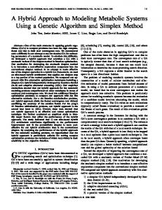
Gene codes.

Fig. 6. Chromosome representation.

control of the corresponding machine. The other one of the generated tokens is in the place dispatch, which implies that the lot must be reworked from the specific operation step. process_ok_ : The transition process_ok_ ( ) is a deterministically timed transition. Similarly, The time delay (processing time) of this transition depends on the current route and step of the lot (token). The firing of process_ok_ represents that the lot just finished the current operation and released the control of the corresponding machine in the th workstation. workstation_ : The place workstation_ ( ) is a place. The number of tokens in workstation_ denotes how many available machines are in the th workstation. The firing of the stochastic transition failure1_ represents the machine failures during idleness, otherwise, the token enables the transition enter_ or enter2_ if necessary. repair_ : The place repair_ ( ) is a place. A token in repair_ represents that a machine in the th workstation is in failure. After some stochastic time period passed, the token in the repair_ can fire the transition repair_ok_ . The time delay used in repair_ok_ depends on the mean time to repair (MTTR). failure1_ , failure2_ and repair_ok_ ( ): These are stochastic transitions. As mentioned above, the time delay used in repair_ok_ depends on the mean time to repair (MTTR), and the time delay used in failure1_ and failure2_ depends on the mean time to fail (MTTF). The firing of the transition failure2_ represents machine failures during an operation. The place workstation_ is initially marked. We model the machine failure probability with the transition failure1_ and failure2_ . If the lot is in processing, the transition failure2_ can be fired. If the machine is in idle state, the transition failure1_ can be fired. Note that the machine cannot fail when being set up in this subnet. The reason for this simplification is that compared to the processing time and idle time, the setup time of machine is relatively short, so that it can be ignored. In addition, if lot is reworked or a machine is in failure while


625

Fig. 7. The architecture of the scheduler.

processing, a token will enter the place dispatch of the routing module. If the lot is successfully processed, a token will enter to place out of Routing module to indicate that the lot is ready for next wafer operation. The case of batch processing machine is somewhat complicated, although its figure is the same as Fig. 4. The color set of enter_ , setup_ , enter2_ , setup_ _ , processing_ , failure_ , process_ok_ , and process_fail_ depends on the batch size of the machine. If the batch size is two, the color set is ; If the batch size is three, the color set is , and so on. We take the case of the batch size 2 as an example, and the differences are described as follows. enter_ (enter2_ ): The transition enter_ (enter2_ ) ) is an immediate transition. Firing this ( transition represents a normal (time-critical operation) batch entering the operation subnet. Two tokens in place buffer_ (be_time_critical_ ) with the color and one token (the color of last in place workstation_ with color operation) will enable the transition enter_ (enter2_ ) with or . After the firing the color of the transition, a token will be assigned into the place setup_ with the color or . Firing this transition represents that the two lots are grouped together. Since we have to memorize the corresponding color of each token (lot) in a batch, we have to expand the length of the color string of the transitions and places mentioned above. in1_ (in2_ ): in1_ (in2_ ) ( ) are the input arcs of the transition enter_ (enter2_ ). The place buffer_ (be_time_critical) with the color

Fig. 8. UltraSim.

has arcs directly connected to the transition with the color and . in3_ (in4_ ): in3_ (in4_ ) ( ) are the input arcs of the transition enter_ (enter2_ ). The place workhas arcs directly connected station_ with the color to the transition with the color . setup_ _ : The transition setup_ _ ( ) is a deterministically timed transition. The function of setup_ _ is

626


Fig. 9. The main window of UltraSim.

to compare the color of the last operation and current operation, i.e., to check whether the corresponding machine in the th workstation needs setup. If the two operations are the same, the corresponding machine does not need setup, and the corresponding batch can be processed immediately. When the color of the transition is , the associated time is zero, and vice , time 0). After the corresponding machine comversa ( pletes setup, the corresponding batch can be processed. out_ : out_ ( ) is the output arc of the transition setup_ _ . The output function can be expressed as an identity matrix in the batch-processing machine and otherwise [ 0]. out2_ (out3_ , out4_ ): out2_ (out3_ , out4_ ) ( ) is the output arc of the transition failure2_ (processing_ok_ , processing_fail_ ). The transition with the color

Fig. 10.

has an arc directly connected to the place repair_ (workstation_ ) with the color . The meaning of firing these transitions is that the last operation performed on this machine is memorized in place workstation_ .

out5_ (out6_ , out7_ ): out5_ (out6_ , out7_ ) ) is the output arc of the transition failure2_ ( (processing_ok_ , processing_fail_ ). The transition with the color

The data access architecture of UltraSim.


Fig. 11.

627

Lot release wizard.

has two (depending on the batch size) arcs directly connected to the place dispatch (out) with and . The meaning of firing these the color transitions is that the batch is separated into lots and ready to do its next operation. IV. WAFER FAB SCHEDULER A typical wafer fabrication facility contains many different products and processes, some with small quantities, competing for resources. Each product flow can contain hundreds of processing steps demanding production time of the same resource many times during the flow. Hence, it is important to develop a production scheduling system that can help to minimize cycle time as well as to maximize the throughput rate and the rate of meeting due dates. Similarly, it is very important to control the release of new lots to the system to avoid starvation of bottlenecks wherever possible. The UNIF (uniform) rule is the most common release control used in wafer fabrication, i.e., release new lots into the fab at a constant rate equal to the desired output rate, but independent of the current inventory level or the machine status. In this paper, we also use UNIF as the lot release control policy, and tune the lot interarrival time to an appropriate value so that the fab can keep a steady WIP level. We can address the following issues in wafer fab [9]: What priorities should be assigned to different jobs competing for the same resource and for late jobs? How to reduce time lost due to setups? Which batching decisions are performed well? How to take machine breakdown into account?

How to avoid rework in some time-critical operations? This is more complex than the traditional job-shop problem. The problem we considered involves reentrant flow, rework, unscheduled machine breakdown, sequence dependent setup times, batch processing machines, and due dates, but we assume the stocker capacity between machines are infinite. GAs were proposed by Holland, whose colleagues and students at the University of Michigan in 1975 used it as a new learning paradigm to model a natural evolution mechanism [17]. Although GAs were not well known in the beginning, after the publication of Goldberg’s book [18], GAs have recently attracted considerable attention in a number of fields such as methodology for optimization, and job-shop scheduling. In this paper, we allow our computation model to support the search algorithm over a CTPN model, i.e., search can be performed in both axes of multiple resources and different time segments. Here, we propose a new scheme to represent a schedule for the problem of production scheduling in wafer fab using GA embedded search over a CTPN model. Before we explain the approach to the GA, we first introduce the following notations. : Population Size. : Number of Generations. : Crossover Rate. : Number of Offsprings. : Mutation Probability. : Inversion Probability. The algorithm starts with an initial set of random configurations called a population, which is a collection of chromosomes. The chromosome here denotes a total scheduling solution for wafer fabrication. The size of the population is always fixed . Following this, a mating pool is established in which pairs

628


TABLE I EQUIPMENT DESCRIPTION

of individuals from the population are chosen. The probability of choosing a particular individual for mating is proportional to its fitness value. Chromosomes with higher fitness values have a greater chance of being selected for mating. Applying crossover to generate new offsprings. Mutation and inversion are also applied with a low probability. Next, the offsprings generated are evaluated on the basis of fitness, and selecting some of the parents and some of the offsprings forms a new generation. The times, where is the number above procedure is executed , the of generations. After a fixed number of generations fittest chromosome, i.e., the one with the highest fitness value is returned as the desired solution. A. Chromosome Representation In this paper, we use priority rule-based representation of chromosomes in the GA. This representation belongs to indirect approaches as described above. With this approach, brings us advantages such as the simplicity of the chromosome structure, simple GA operators, and shorter computation time. First, we define a gene as follows. A gene set is used to indicate the scheduling policy over the CTPN model. That is, each machine group (identical machines) has a gene is a 3-tuple where associated with it. A gene

: one type of dispatching rules. : one type of setup rules. : one type of batching rules. The rules we selected for gene codes are listed in Fig. 5. For each rule, it is described as follows: FCFS: First Come First Serve. MINS: Minimum Inventory at the Next Station first. In this rule, a lot has a higher priority if its next operation workstation has a lower inventory. SRPT: Shortest Remaining Processing Time first. EDD: Earliest Due Date first. SSU: Same Set-Up first. W1T: Waiting for the arrival lot to complete the batch within one unit of lot interarrival time. When the batch is completed within this specific period, the batch is started immediately. Otherwise, the partial batch is started right after one unit of lot interarrival time. W2T: The same as W1T, but the maximum waiting for completing a batch is two units of lot interarrival time. W3T: The same as W1T, but the maximum waiting for completing a batch is three units of lot interarrival time. W4T: The same as W1T, but the maximum waiting for completing a batch is four units of lot interarrival time. The dispatching rules, setup rules and batching rules are directly related to the Elementary Module of the CTPN model.


629

TABLE II PROCESS FLOW FOR ROUTE 1

The dispatching rules and set-up rules are associated with the transition enter_ and enter2_ . Each time when there are more than one token in place buffer_ (or be_time_critical_ ) and the machine is idle, the scheduler must select one of the tokens (lots) to process. This selection depends on the rules it used. For example, if set-up rule “SSU” and dispatching rule “FCFS” is selected, it will first select the tokens with the same operation type

of the last lot processed on machine. Then, we select among them using FCFS rule, the lot entering the queue with the earliest time will be selected first. The batching rule that we called dynamic batch-size rule will automatically calculate the most suitable waiting time to complete a batch. Normally, the batch size of each machine is fixed so that, when the partial batch will be processed, the system will

630


TABLE III PROCESS FLOW FOR ROUTE 2

automatically insert dummy lots (or wafers) to the partial batch to complete a batch. After genes are defined, the chromosome can be created. In this paper, the length of a chromosome is fixed, and is equivalent to the number of machine groups. The structure of the chromosome is depicted in Fig. 6.

chromosome (i.e., solution); combined fitness function; th objective function; constant weight for ; number of the objective functions. We use two objective functions in our implementation. The fitness function is defined as follows:

B. Fitness Function One of the simplest methods to combine multiple objective functions into a scalar fitness solution is the following weighted sum approach:

where

where is the score for mean cycle time and is the score for number of lots which meet due date. Before evaluating the fitness function, and must be determined first. We calculate and by the following way: For , sort all the chromosomes by mean cycle time, and give each chromosome a rank such that the one with shorter mean cycle


631

TABLE IV PROCESS FLOW FOR ROUTE 3

time can get a higher rank. For example, we now have 4 chroand and mosomes

where

Therefore,

assume that we have fivechromosomes , and , and each chromosome leads to the following values:

is the mean cycle time, then

If For , sort all the chromosomes by the number of lots which meet the due date, and give each chromosome a rank such that the more number of lots which meet the due date can get a higher rank. and are transformed into Note that the functions functions with discrete rank values. The purpose of this transin the fitness formation is to make the selection of the value function more easily. After transformation, the value of cycle time and meet-due-date rate can fall into the same range (in with the value following example 1 5). Then if we assign larger than , which means the cycle time is more important than meet-due-date rate in fitness function, and vice versa.

Thus,

, then

or

is the best chromosome.

C. Genetic Operators Crossover: Crossover is the main genetic operator. It operates on two individuals and generates an offspring. It is an inheritance mechanism where the offspring inherits some of the characteristics of the parents. The operation consists of choosing a random cut point and generating the offspring by combining the

632


TABLE V THREE ORDERS

TABLE VII THE COMPARED RESULT FOR CASE 1

TABLE VI THE CONTENTS OF THE CHROMOSOME

TABLE VIII FOUR ORDERS TO BE RELEASED INTO THE FAB

TABLE IX THE COMPARED RESULT FOR CASE 2

segment of one parent to the left of the cut point with the segment of the other parent to the right of the cut. Mutation: Mutation produces incremental random changes in the offspring generated by the crossover. The commonly used mutation mechanism is pairwise interchange. We also use this mechanism in our implementation. Fig. 8 shows an example. Inversion: We add an additional genetic operator called inversion [16] in the implementation. In the inversion operation, two points are randomly chosen along the length of the chromosome so that the order of genes within the two end points of the chromosome reverses. D. Schedule Builder A schedule builder is dedicated to transforming a chromosome to a feasible schedule, such that we can evaluate the aforementioned indirect chromosome representation. Based on the CTPN model, the evolution of the system can be addressed by the change of marking in the net. Consequently, all possible kinds of behavior of the system can be completely tracked by the reachability graph of the net. In other words, we can track the WIP status from the CTPN model while the schedule was performed. A chromosome consists of many genes, each of which consists of rules which are directly related to the Elementary Module of CTPN model. Thus, given a CTPN model and a chromosome, the schedule builder can generate a feasible schedule that consists of the firing se-

quence of the transitions, which provides the order of the initiation of operations. In the following algorithm, we describe how a schedule builder uses the chromosome to construct a feasible schedule over the CTPN model. One simulation of the whole model carried out for the policy that corresponds to the chromosome. Once the scheduling environment is changed, the scheduler builder will be executed. The architecture of the scheduler was shown in Fig. 7, in which, we first select a lot release policy to control the timing for release of a lot (token) to the CTPN model. Second, apply the GA over the CTPN to find a good chromosome. Algorithm 1 Schedule Builder Begin ; Select a chromosome Apply the scheduling rules to the according genes; as the initial Set the marking ; marking Find the set of all enabled transitions ; in the marking , namely


Fig. 12.

633

Performance evaluation for mean queuing time in case 1.

While is not the final marking Do Then If Update the elapsing time; as the current Set the marking marking ; ; Update Else Do For all by according Fire the transition scheduling rules if necessary;(if is associated with the transition rule, we have to check which color of this transition can be fired first to resolve the conflict) as the current Set the marking new marking ; ; Update End For End IF End While End. V. IMPLEMENTATION In order to implement the systematic wafer fab modeling as well as the scheduling method, we develop a simulation tool called UltraSim (see Fig. 8) that was designed by an object oriented method and programming with C++ in Microsoft Visual C++ 6.0. In Fig. 9, it is a main window of the UltraSim. The additional function of UltraSim is that it can access the remote shared database through ODBC (open database connectivity) manager. The remote shared database here, is implemented by Microsoft SQL Server 6.5. Fig. 10 is the remote data access architecture between UltraSim and SQL Server. Through the remote database, we can easily get the WIP status for simulation. This is so convenient that we do not need to run the model from the empty fab, and, the results of simulation will be more close to a real fab. Besides the remote shared database, which can be used in UltraSim, we can also save/load our model and

WIP status to/from files. This characteristic makes UltraSim applicable almost everywhere, even if the network does not function. Moreover, UltraSim provides a friendly user interface to help users to create a CTPN model. In addition, UltraSim has a lot release wizard to help customers to insert their orders easily. In Fig. 11, we have two choices to select scheduling policies to be applied to the production scheduling. The two kinds of scheduling policies are simple dispatching rules and genetic algorithm scheduler. If we select simple dispatching rules, we must select one of the four dispatching rules in advance. After the operation on the lot release wizard is finished, the selected scheduling policy will be shown in status bar under the main window. Moreover, if results is good enough compared to the popular schedule rules, then, the GA search is stopped. VI. EXPERIMENT RESULTS The simulation model we used in this paper is based on Wein’s model [1]. It describes a fictitious wafer fab, but most of the parameters of the model are derived from data gathered at the Hewlett-Packard Technology Research Center Silicon fab (the TRC fab), which is a large R&D facility in Palo Alto, CA. Unlike the model studied by Wein [1], we enlarge the capacity of the fab to increase the complexity of the simulation. Moreover, we add the rework probability to the inspection machines, and define the reworked step in each route. Batch processing machines are also included in our simulation model, so that the simulation model can be close to real fab. We assume both of the workstations of TMNOX and PLM6 are batch-processing machines, and their batch sizes are 4 and 2, respectively. The whole equipment information of the simulation fab is listed in Table I, which describes the detailed parameters of the fab, such as mean processing time (MPT), mean set-up time (MST), mean time to repair (MTTR), and mean time between failure (MTBF). In the simulation model, the machine downtime that consists of unscheduled breakdowns. Time between failures and time to repair for each workstation is randomly generated from uniform

634

Fig. 13.


Performance evaluation for meeting due date in case 1.

Fig. 14. Performance evaluation for mean queuing time in case 2.

distributions with given mean values in implementation. In TRC fab model, the MPT contains the mean processing time and mean set-up time, but we separate them in our simulation model. The MPT in our simulation model is equal to 0.9 MPT in TRC fab model, and the MST is equal to 0.1 MPT in TRC fab model. In our simulation model, each lot entering the fab is based on a specific process flow. There are three different process flows in our simulation model, and the sequence of stations to be visited in three process flows are listed in Tables II–IV, respectively, where the numbers refer to the station numbers in the first column of Table I. The process flow for route 1 listed in Table II is the same as the one earlier studied by Wein [1], which requires 12 loops, i.e., a lotvisitslithographyexposureworkstations12times.Theprocess flow for route 2 and route 3 is generated by randomly selecting 10 loops and 8 loops from route 1, respectively. We assume the re-entrance of operation on the same machine may have different processing time, since they have different recipes to be processed. In addition, if the machine takes processes with different recipes, the machine must be set-up. Here,

the processing time (PT) for a lot is randomly generated from a uniform distribution between 0.9 MPT and 1.1 MPT, where MPT is given for each station in Table I. It is likewise for the set-up time (ST), which is randomly generated from a uniform distribution between 0.9 MST and 1.1 MST, where MST is given for each station in Table I. In our experiments, the average population size is 10, the average generation size is 10, the crossover rate is 0.7, the mutation probability is 5%, and inversion probability is 1%. Case 1: Three Orders for Total 100 Lots: The problem description is listed in Table V, and the chromosome searched by GA scheduler is listed in Table VI, where the rules listed in the chromosome can be referred to Fig. 5 in Section III. Note that if workstations do not perform batch-processing operation, their corresponding batch rules are useless. For the four simple dispatching rules, the maximum waiting time to complete a batch is 24 hours. The lot interarrival time we used in this simulation is 12 hours for all the scheduling policies, since this lot interarrival time can build a steady WIP level for our simulation model.


Fig. 15.

635

Performance evaluation for meeting due date in case 2.

We evaluated the performance of the five scheduling policies, which are FCFS, SRPT, MINS, EDD, and GA. In addition, the four simple dispatching rules plus SSU are also evaluated. For each scheduling policy, we run 10 times of simulation and calculate mean value and standard deviation. The compared results are listed in Table VII, where the two criteria are mean queuing time (MQT) and the rate of meeting due date (MDD). The total computation time of case 1 is 23 minutes (on Pentium II 450MHz with 128MB SDRAM). Case 2: Four Orders for Total 80 Lots: Unlike the case 1, we have four orders in the case 2. In addition, the route sequence we used as the input pattern in the case 2 is different from the case 1. However, the chromosome used in the case 2 is the same as one used in the case 1, i.e., we did not re-schedule to search for the new chromosome given for the new input pattern. The purpose of using the same chromosome is to test whether the pre-searched chromosome can be applicable under different input patterns and can still perform well. As for other conditions, they are made the same as in case 1. Here we listed the four orders, and one compared result in Tables VIII and IX, respectively. The total computation time of case 2 is 20 minutes (on Pentium II 450MHz with 128MB SDRAM). From Figs. 14 and 15, we found that the proposed GA scheduler performs much better than other conventional dispatching rules. It has a lower queuing time for lots spent in the fab, a higher rate for meeting the customers’ due date. In addition, the experimental results show that the proposed GA scheduler has a lower variability on the total queuing time and the rate of meeting duedate, which increases the accuracy of the simulation based prediction. As a result, the proposed GA scheduler has a significant impact on wafer fab scheduling, by providing obvious improvements over the other conventional dispatching rules, even though the fab has a mixed production. VII. CONCLUSION In this paper, we consider the wafer fab scheduling problem. We first proposed a systematic CTPN model for a wafer fab. The

entire CTPN model is composed of two modules, one is routing module, and the other is elementary module. Then, in order to make better scheduling policies on wafer fab, we proposed a genetic algorithm scheduler, which dynamically searches for the appropriate dispatching rules for each machine group or processing unit family. Through the experiments, we found that the GA scheduler provides more superior performance than the conventional dispatching rules do. In implementation, we developed a simulation tool for modeling and scheduling for wafer fab. The simulation tool, called UltraSim, provides a friendly user interface to help users to model their fab easily, and provides an efficient method to search for a better solution on wafer fab scheduling by using genetic algorithm. REFERENCES [1] L. M. Wein, “Scheduling semiconductor wafer fabrication,” IEEE Trans. Semicond. Manufact., vol. 1, pp. 115–130, 1988. [2] C. R. Glassey and M. C. Resende, “Closed-loop job release control for VLSI circuit manufacturing,” IEEE Trans. Semicond. Manufact., vol. 1, pp. 36–46, 1988. [3] H. Chen, J. M. Harrison, A. Mandelbaum, A. V. Ackere, and L. M. Wein, “Empirical evaluation of a queuing network model for semiconductor wafer fabrication,” Operat. Res., vol. 36, no. 2, pp. 202–215, 1988. [4] C. R. Glassey and W. W. Weng, “Dynamic batching heuristic for simultaneous processing,” IEEE Trans. Semicond. Manufact., vol. 4, pp. 77–82, 1991. [5] R. Uzsoy, L. A. Martin-Vega, C. Y. Lee, and P. A. Leonard, “Production scheduling algorithm for a semiconductor test facility,” IEEE Trans. Semicond. Manufact., vol. 4, pp. 270–279, 1991. [6] R. Uzsoy, C. Y. Lee, and L. A. Martin-Vega, “A review of production planning and scheduling models in the semiconductor industry—Part I: System characteristics, performance evaluation and production planning,” IIE Trans., vol. 24, no. 4, pp. 47–60, 1992. [7] P. K. Johri, “Practical issues in scheduling and dispatching in semiconductor wafer fabrication,” J. Manufact. Syst., vol. 12, no. 6, pp. 474–485, 1993. [8] R. Uzsoy, C. Y. Lee, and L. A. Martin-Vega, “A review of production planning and scheduling models in the semiconductor industry—Part II: Shop-floor control,” IIE Trans., vol. 26, no. 5, pp. 44–55, 1994. [9] L. Duenyas, J. W. Fowler, and L. W. Schruben, “Planning and scheduling in Japanese semiconductor manufacturing,” J. Manufact. Syst., vol. 13, no. 5, pp. 323–332, 1994. [10] S. Li, T. Tang, and D. W. Collins, “Minimum inventory variability schedule with applications in semiconductor fabrication,” IEEE Trans. Semicond. Manufact., vol. 9, pp. 145–149, 1996.

636


[11] Y. Narahari and L. M. Khan, “Modeling the effect of hot lots in semiconductor manufacturing systems,” IEEE Trans. Semicond. Manufact., vol. 10, pp. 185–188, 1997. [12] Y. D. Kim, J. U. Kim, S. K. Lim, and H. B. Jun, “Due-date based scheduling and control policies in a multiproduct semiconductor wafer fabrication facility,” IEEE Trans. Semicond. Manufact., vol. 11, no. 1, pp. 155–164, 1998. [13] Y. D. Kim, D. H. Lee, and J. U. Kim, “A simulation study on lot release control, mask scheduling, and batch scheduling in semiconductor wafer fabrication facilities,” J. Manufact. Syst., vol. 17, no. 2, pp. 107–117, 1998. [14] S. A. Mosley, T. Teyner, and R. M. Uzsoy, “Maintenance scheduling and staffing policies in a wafer fabrication facility,” IEEE Trans. Semicond. Manufact., vol. 11, no. 2, pp. 316–323, 1998. [15] S. M. Sze, VLSI Technology. New York: McGraw-Hill, 1983. [16] S. M. Sait and H. Youssef, VLSI Physical Design Automation: Theory and Practice. New York: McGraw-Hill, 1995. [17] J. H. Holland, Adaptation in Natural and Artificial Systems: Michigan Univ. Press, 1975. [18] D. E. Goldberg, Genetic Algorithm in Search, Optimization and Machine Learning. Reading, MA: Addison-Wesley, 1989. [19] R. Cheng, M. Gen, and Y. Tsujimura, “A tutorial survey of job-shop scheduling problems using genetic algorithm—Part I: Representation,” Comput. Indust. Eng., vol. 30, no. 4, pp. 983–997, 1996. [20] C. Y. Lee, S. Piramuthu, and Y. K. Tsai, “Job shop scheduling with a genetic algorithm and machine learning,” Int. J. Prod. Res., vol. 35, no. 4, pp. 1171–1191, 1997. [21] R. S. Lee and M. J. Shaw, “A genetic algorithm-based approach to flexible flow-line scheduling with variable lot sizes,” IEEE Trans. Syst., Man, Cybern. B, vol. 27, pp. 36–54, 1997. [22] G. Ulusoy, S. S. Funda, and U. Bilge, “A genetic algorithm approach to the simultaneous scheduling of machines and automated guided vehicles,” Comput. Operat. Res., vol. 24, no. 4, pp. 335–351, 1997. [23] J. L. Peterson, Petri Net Theory and the Modeling of Systems: McGrawHill, 1981. [24] A. A. Desrochers and R. Y. Al-Jaar, Applications of Petri Nets in Manufacturing Systems: Modeling, Control, and Performance Analysis. New York: IEEE Press, 1994. [25] M. H. Lin and L. C. Fu, “Modeling, analysis, simulation, and control of semiconductor manufacturing systems: A generalized stochastic colored-timed Petri-net approach,” in IEEE Int. Conf. Syst., Man, Cybern., 1999. [26] R. Zurawski and M. C. Zhou, “Petri nets and industrial applications: A tutorial,” IEEE Trans. Industrial Electron., vol. 41, pp. 567–583, 1994. [27] M. C. Zhou and M. D. Jeng, “Modeling, analysis, simulation, scheduling, and control of semiconductor manufacturing systems: A Petri net approach,” IEEE Trans. Semicond. Manufact., vol. 11, pp. 333–357, 1998. [28] M. D. Jeng, X. Xie, and S. W. Chou, “Modeling, qualitative analysis, and performance evaluation of the etching area in an IC wafer fabrication system using Petri nets,” IEEE Trans. Semicond. Manufact., vol. 11, pp. 358–373, 1998. [29] H. H. Xiong and M. C. Zhou, “Scheduling of semiconductor test facility via Petri nets and hybrid heuristic search,” IEEE Trans. Semicond. Manufact., vol. 11, pp. 384–393, 1998. [30] S. Y. Lin and H. P. Huang, “Modeling and emulation of a furnace in IC fab based on colored-timed Petri net,” IEEE Trans. Semicond. Manufact., vol. 11, pp. 410–420, 1998. [31] K. Jensen, “Colored Petri nets and the invariant method,” in Theoretical Computer Science. Amsterdam: North-Holland, 1981, vol. 14, pp. 317–336.

Jyh-Horng Chen received the M.S. degree from National Taiwan University, Taipei, Taiwan, R.O.C., in 1999. His research interests include modeling, simulation, and scheduling of manufacturing systems. He joined TSMC, the largest domestic semiconductor company, as an engineer immediately following graduation.

Li-Chen Fu was born in Taipei, Taiwan, R.O.C., in 1959. He received the B.S. degree from National Taiwan University, Taipei, Taiwan, in 1981, and the M.S. and Ph.D. degrees from the University of California, Berkeley, in 1985 and 1987, respectively. Since 1987, he has been a professor with both the Department of Electrical Engineering and the Department of Computer Science and Information Engineering of National Taiwan University. He currently also serves as the Deputy Director of Tjing Ling Industrial Research Institute of National Taiwan University. His areas of research interest include robotics, FMS scheduling, shop floor control, home automation, visual detection and tracking, E-commerce, and control theory and applications. Dr. Fu is a member of the IEEE Robotics and Automation Society and Automatic Control Society. He is also a member of the Board of the Chinese Automatic Control Society and the Chinese Institute of Automation Engineers. During 1996–1998 and 2000, he was appointed a member of AdCom of IEEE Robotics and Automation Society, and will serve as the Program Chair of 2003 IEEE International Conference on Robotics and Automation. He has been Editor of Journal of Control and Systems Technology and an Associate Editor of the prestigious control journal, Automatica. Since 1999, he has been Editor-in-Chief of a new control journal, the Asian Journal of Control.

Ming-Hung Lin (M’88) received the M.S. and Ph.D. degrees from National Taiwan University, Taipei, Taiwan, R.O.C., in 1993 and 2001, in computer science and information engineering, respectively. Since 1995, he has been with Computer Communication Research Labs., Industrial Technology Research Institute (ITRI), where he is researcher on advanced broadband wired and wireless communication systems. He has been involved in several system prototypes such as PC-based video-on-demand, mobile Internet system, and RLC/MAC protocol for GPRS/UMTS. He joined Philips Research East Asia in December 1999, where he is working on information appliance systems. His current research interests include wireless connectivity for home and away environment (Bluetooth and UMTS), mobile multimedia systems, VLSI design for mobile display system, hybrid queuing theorem, and automatic production research.

An-Chih Huang received the B.S. and M.S. degrees from National Taiwan University, Taipei, Taiwan, R.O.C., in 1999 and 2001, respectively. His research interests include modeling, simulation, prediction, and scheduling of manufacturing systems. He is currently fulfilling his military service.